Improving AHG Estimates

library(AHGestimation)
data <-  select(nwis, date, Q = Q_cms, Y = Y_m, TW = TW_m, V = V_ms)

Increasing AHG skill:

In the last section we saw the traditional OLS based fit on our sample data provided a solution that met continuity, but, has a large amount of error. In this section we will explore alternative methods to see

Curve Fitting Approaches

When fitting a nonlinear curve to a set of data, the options are: (1) linearize the relationship by transforming the data; (2) fit a polynomial spline to the data; or (3) fit a nonlinear function. With our emphasis on interoperable power law relations, only the linear (1) and nonlinear (3) approaches are appropriate.

Nonlinear Least Square (NLS) regression provides more flexible curve fitting through an iterative optimization. NLS approaches require a specified starting value for each unknown parameter to ensure the solver converges on a global rather than a local minimum. When suboptimal starting values are provided, NLS solvers may converge on a local minimum, or, not at all.

OLS

ols <- function(X, Y, name = NA){
  fit <- lm(log(Y) ~ log(X))
  data.frame(coef = exp(fit$coefficients[1]),
             exp  = fit$coefficients[2],
             name = name,
             row.names = NULL)
}

(ols_fit <- bind_rows(
        ols(data$Q, data$Y, "Y"),
        ols(data$Q, data$TW, "TW"),
        ols(data$Q, data$V, "V"))%>% 
    mutate(method = "ols"))
#>         coef       exp name method
#> 1  0.2018376 0.4794202    Y    ols
#> 2 22.6153841 0.1145234   TW    ols
#> 3  0.2178592 0.4056932    V    ols

sum(ols_fit$exp)
#> [1] 0.9996368
prod(ols_fit$coef)
#> [1] 0.9944476

olsP <- data %>% 
  mutate(Yp  = ols_fit$coef[1] * (Q ^ ols_fit$exp[1]),
         TWp = ols_fit$coef[2] * (Q ^ ols_fit$exp[2]),
         Vp  = ols_fit$coef[3] * (Q ^ ols_fit$exp[3]))
         
ols_e <- data.frame(
  Ye  = nrmse(olsP$Y, olsP$Yp),
  TWe = nrmse(olsP$TW, olsP$TWp),
  Ve  = nrmse(olsP$V, olsP$Vp)) %>% 
  mutate(tot_error = Ye + TWe + Ve, type = "OLS")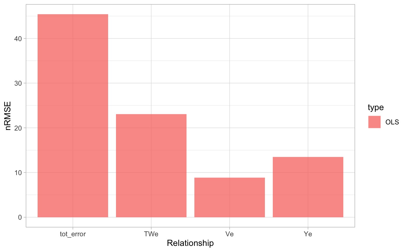

NLS

nls <- function(X, Y, coef, exp, name = NA){
  s <-  summary(suppressWarnings({
    stats::nls(Y ~ alpha * X ^ x,
        start = list(alpha = coef, x = exp), 
        trace = FALSE,
        control = nls.control(maxiter = 50, tol=1e-09,  warnOnly=TRUE))
  }))
  
  data.frame(coef = s$coefficients[1,1],
             exp  = s$coefficients[2,1],
             name = name,
             row.names = NULL)
}

(nls_fit <- bind_rows(
        nls(X = data$Q, 
            Y = data$Y,  
            coef = ols_fit$coef[1], 
            exp = ols_fit$exp[1],
            "Y"),
        nls(X = data$Q, 
            Y = data$TW, coef = ols_fit$coef[2], 
            exp = ols_fit$exp[2], 
            "TW"),
        nls(X = data$Q, 
            Y = data$V,  coef = ols_fit$coef[3], 
            exp = ols_fit$exp[3], 
            "V")) %>% 
    mutate(method = "nls"))
#>         coef       exp name method
#> 1  0.1867125 0.5190562    Y    nls
#> 2 22.7934449 0.1166774   TW    nls
#> 3  0.2898890 0.3246968    V    nls

sum(nls_fit$exp)
#> [1] 0.9604304
prod(nls_fit$coef)
#> [1] 1.233716

nlsP <- data %>% 
  mutate(Yp  = nls_fit$coef[1] * (Q ^ nls_fit$exp[1]),
         TWp = nls_fit$coef[2] * (Q ^ nls_fit$exp[2]),
         Vp  = nls_fit$coef[3] * (Q ^ nls_fit$exp[3]),
         method = "nls")
         
nls_e <- data.frame(
  Ye  = nrmse(nlsP$Y, nlsP$Yp),
  TWe = nrmse(nlsP$TW, nlsP$TWp),
  Ve  = nrmse(nlsP$V, nlsP$Vp)
) %>% 
  mutate(tot_error = Ye + TWe + Ve, type = "NLS")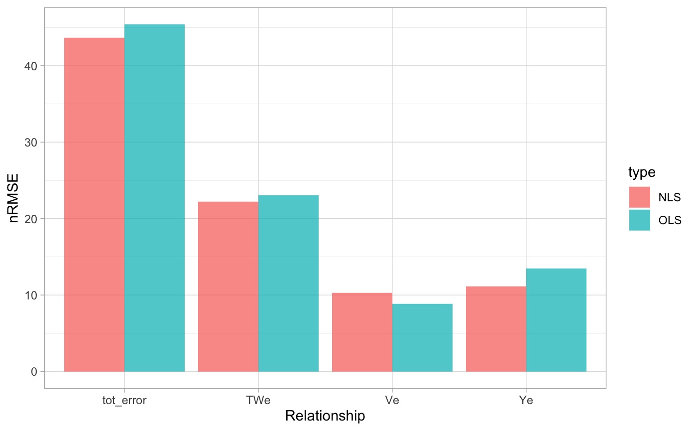

NSGA-II

allowance <- 0.05

# x assumed to be ordered as: k, m, a, b, c, f
objective_function <- function(x) {
      v <- nrmse(x[1]*data$Q^x[2], data$V) 
      t <- nrmse(x[3]*data$Q^x[4], data$TW) 
      d <- nrmse(x[5]*data$Q^x[6], data$Y) 
      return(c(v,t,d))
}

constraint <- function(x) {
    return(c((1 + allowance) - (x[1] * x[3] * x[5]),
             (x[1] * x[3] * x[5]) - (1 - allowance),
             (1 + allowance) - (x[2] + x[4] + x[6]),
             (x[2] + x[4] + x[6]) - (1 - allowance)))
}

set.seed(10291991)

res <- nsga2(
      objective_function,
      constraints   = constraint,
      # 6 inputs, 3 outputs, 4 constraints
      idim = 6, odim = 3, cdim = 4,
      # Bounds determined from literature
      lower.bounds  = c(0, 0, 0, 0, 0, 0),
      upper.bounds  = c(3.5, 1, 642, 1, 20, 1),
      # Defaults we've chosen
      generations   = 200,
      popsize       = 32,
      cprob = .5,
      mprob = .1)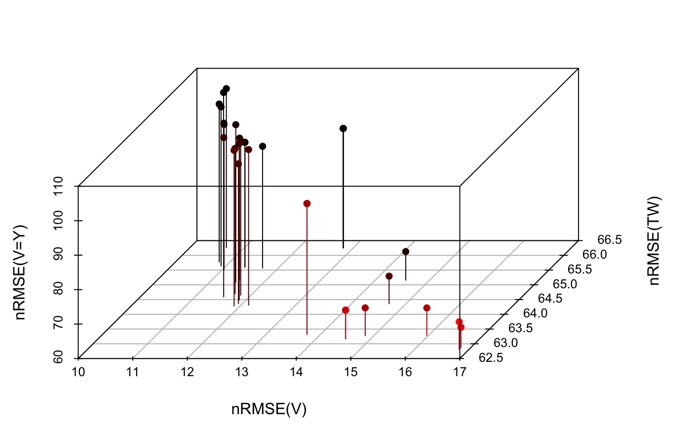

vals <- res$value[res$pareto.optimal, ]
vals <- vals[!duplicated(vals), ]

par  <- res$par[res$pareto.optimal, ]
par  <- par[!duplicated(par), ]

ahg <- par[which.min(rowSums(vals)),]

nsga_fit <- data.frame(coef = ahg[c(1,3,5)], exp = ahg[c(2,4,6)], 
                       name = c("V", "TW", "Y"), 
                       method = "nsga2")

nsgs_e <- data.frame(
  Ve = nrmse((ahg[1] * data$Q ^ ahg[2]), data$V) ,
  TWe = nrmse((ahg[3] * data$Q ^ ahg[4]), data$TW), 
  Ye = nrmse((ahg[5] * data$Q ^ ahg[6]), data$Y),
  type = "nsga2") %>% 
  mutate(tot_error = Ve + TWe + Ye)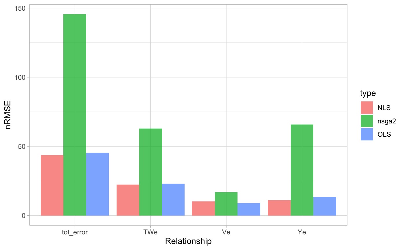

Combination Approach

d <- bind_rows(ols_fit, nls_fit, nsga_fit)
r <- split(d, f = d$name)  

fit <-  function(g, ind, V, TW, Y, Q, allowance = .05) {
    x <- g[ind,]
    g$V_error[ind] <-  nrmse(x$V_coef*(Q^x$V_exp), V)
    g$TW_error[ind] <- nrmse(x$TW_coef*(Q^x$TW_exp), TW)
    g$Y_error[ind] <-  nrmse(x$Y_coef*(Q^x$Y_exp), Y) 
    c1 <- round(g$V_coef[ind] * g$Y_coef[ind] * g$TW_coef[ind], 3)
    c2 <- round(g$V_exp[ind] + g$Y_exp[ind] + g$TW_exp[ind], 3)
    g$viable[ind] <-  (between(c1, 1-allowance, 1+allowance) +  
                       between(c2, 1-allowance, 1+allowance)) == 2
    return(g)
}
    
names <- c("V", "TW", "Y")

g <- rep(list(c("ols", "nls", "nsga2")), 3) %>% 
    expand.grid() %>% 
    setNames(paste0(names, "_method")) %>% 
    mutate(viable = NA, tot_error = NA) %>% 
    bind_cols(setNames(data.frame(matrix(NA, ncol = 9, nrow =27)), 
                          c(paste0(names, "_error"), 
                            paste0(names, "_coef"), 
                            paste0(names, "_exp"))))

  
for(t in 1:3){
    x <- g[[paste0(names[t], "_method")]]
    ind <- match(x, r[[names[t]]]$method)
    
    g[[paste0(names[t], '_exp')]] <- r[[names[t]]]$exp[ind]
    g[[paste0(names[t], '_coef')]] <- r[[names[t]]]$coef[ind]
}

for(i in seq(nrow(g))){ g <- fit(g, i, data$V, data$TW, data$Y, data$Q)}

g$tot_error <- rowSums(g[, grepl("error", names(g))], na.rm = TRUE)

combo <- filter(g, viable == TRUE) %>% 
      slice_min(tot_error) %>% 
      mutate(condition = "bestValid")
    
ols <- filter(g, Y_method == "ols", TW_method == "ols", V_method == "ols") %>% 
      mutate(condition = "ols")
    
nls <- filter(g, Y_method == "nls", TW_method == "nls", V_method == "nls") %>% 
      mutate(condition = "nls")
  
nsga <- filter(g, 
               Y_method == "nsga2", 
               TW_method == "nsga2", 
               V_method == "nsga2") %>% 
        mutate(condition = "nsga2")

summary <- bind_rows(combo, ols, nls, nsga) %>%  
          arrange(!viable, tot_error)

V_method	TW_method	Y_method	viable	tot_error	V_error	TW_error	Y_error	V_coef	TW_coef	Y_coef	V_exp	TW_exp	Y_exp	condition
ols	nls	ols	TRUE	31.98	10.93	12.94	8.11	0.22	22.79	0.20	0.41	0.12	0.48	bestValid
ols	ols	ols	TRUE	32.03	10.93	12.99	8.11	0.22	22.62	0.20	0.41	0.11	0.48	ols
nsga2	nsga2	nsga2	TRUE	145.60	16.82	62.87	65.91	0.57	0.41	4.14	0.18	0.86	0.00	nsga2
nls	nls	nls	FALSE	30.82	9.98	12.94	7.90	0.29	22.79	0.19	0.32	0.12	0.52	nls

Packaged Functionality

The above workflow follows this diagram:

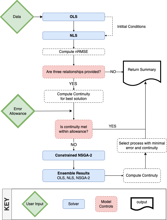
And can be executed like this:

ahg <- ahg_estimate(data)

NOTE Single relationships can also be fit like this:

ahg_estimate(select(data, Q, Y))
#>   type       exp      coef nrmse    pb method
#> 1    Y 0.5190562 0.1867125  7.90 -0.23    nls
#> 2    Y 0.4794202 0.2018376  8.11 -5.58    ols

Mike Johnson

Increasing AHG skill:

Curve Fitting Approaches

OLS

NLS

NSGA-II

Combination Approach

Packaged Functionality