Lab 2: Distances and Projections

Hints & Tricks

Question 1:

Making Spatial Objects & Coordinate Transformation

Spatial objects (sf) can be built from a vector of X and Y values in addition to a coordinate reference system (CRS). For example:

df <- data.frame(name = state.name, 
                X = state.center$x, 
                Y = state.center$y)
head(df)

        name         X       Y
1    Alabama  -86.7509 32.5901
2     Alaska -127.2500 49.2500
3    Arizona -111.6250 34.2192
4   Arkansas  -92.2992 34.7336
5 California -119.7730 36.5341
6   Colorado -105.5130 38.6777

# Geographic Coordinate System (GCS)
(df_sf_gcs = st_as_sf(df, 
                      coords = c("X", "Y"), 
                      crs = 4269))

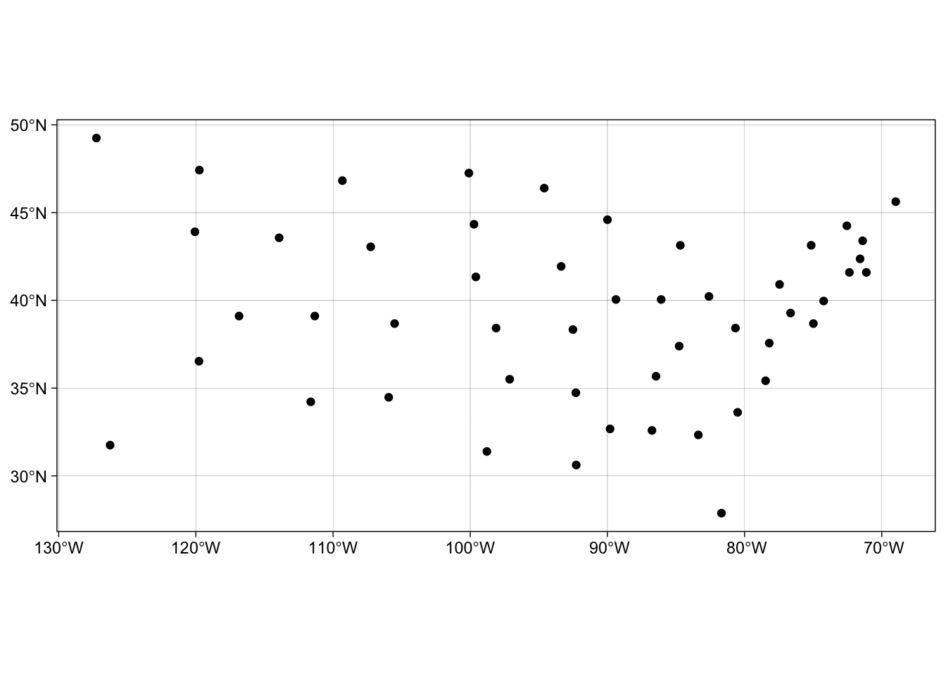
Simple feature collection with 50 features and 1 field
Geometry type: POINT
Dimension:     XY
Bounding box:  xmin: -127.25 ymin: 27.8744 xmax: -68.9801 ymax: 49.25
Geodetic CRS:  NAD83
First 10 features:
          name                 geometry
1      Alabama POINT (-86.7509 32.5901)
2       Alaska    POINT (-127.25 49.25)
3      Arizona POINT (-111.625 34.2192)
4     Arkansas POINT (-92.2992 34.7336)
5   California POINT (-119.773 36.5341)
6     Colorado POINT (-105.513 38.6777)
7  Connecticut POINT (-72.3573 41.5928)
8     Delaware POINT (-74.9841 38.6777)
9      Florida  POINT (-81.685 27.8744)
10     Georgia POINT (-83.3736 32.3329)

ggplot() + 
  geom_sf(data = df_sf_gcs) + 
  coord_sf(datum = st_crs(df_sf_gcs)) +
  theme_linedraw()

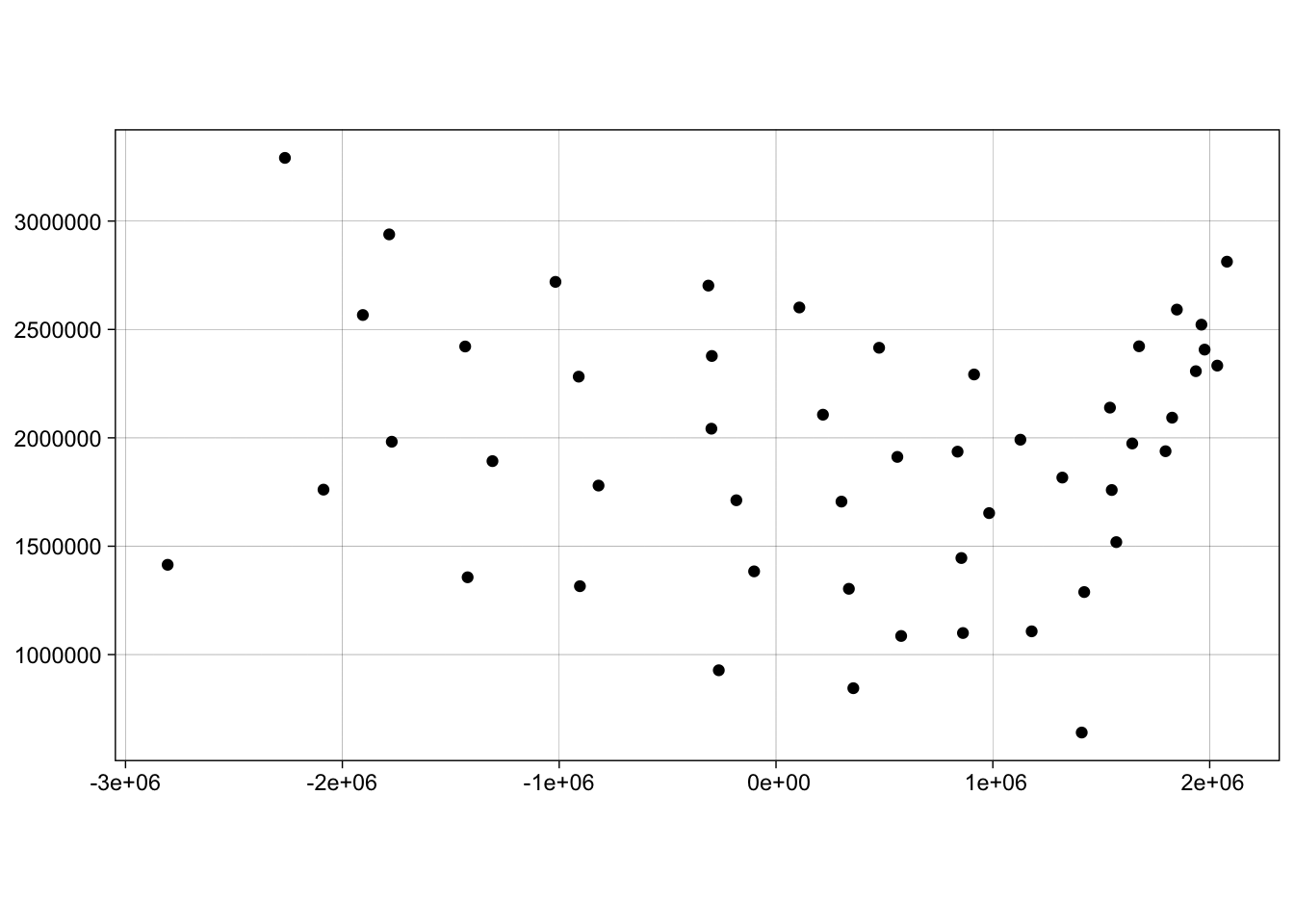
# Projected Coordinate System (PCS)
# st_transforms converts from one reference system to another
(df_sf_pcs = st_transform(df_sf_gcs, 5070))

Simple feature collection with 50 features and 1 field
Geometry type: POINT
Dimension:     XY
Bounding box:  xmin: -2805703 ymin: 640477 xmax: 2079664 ymax: 3291437
Projected CRS: NAD83 / Conus Albers
First 10 features:
          name                  geometry
1      Alabama  POINT (862043.5 1099545)
2       Alaska  POINT (-2264853 3291437)
3      Arizona  POINT (-1422260 1356663)
4     Arkansas  POINT (336061.5 1303543)
5   California  POINT (-2086972 1760961)
6     Colorado POINT (-818480.9 1779785)
7  Connecticut   POINT (1936213 2307450)
8     Delaware   POINT (1796466 1938236)
9      Florida    POINT (1409814 640477)
10     Georgia   POINT (1179012 1107322)

ggplot() + 
  geom_sf(data = df_sf_pcs) + 
  coord_sf(datum = st_crs(df_sf_pcs)) +
  theme_linedraw()

Question 2:

`st_distance` review

# Three most populous cities in the USA
(big3 = cities |> 
   select(city, population) |> 
   slice_max(population, n = 3))

Simple feature collection with 3 features and 2 fields
Geometry type: POINT
Dimension:     XY
Bounding box:  xmin: -2032603 ymin: 1468468 xmax: 1833394 ymax: 2178657
Projected CRS: NAD83 / Conus Albers
# A tibble: 3 × 3
  city        population           geometry
  <chr>            <dbl>        <POINT [m]>
1 New York      18832416  (1833394 2178657)
2 Los Angeles   11885717 (-2032603 1468468)
3 Chicago        8489066 (684628.3 2122698)

# Fort Collins
(foco = filter(cities, city == "Fort Collins") |> 
    select(city, population))

Simple feature collection with 1 feature and 2 fields
Geometry type: POINT
Dimension:     XY
Bounding box:  xmin: -760147.5 ymin: 1984620 xmax: -760147.5 ymax: 1984620
Projected CRS: NAD83 / Conus Albers
# A tibble: 1 × 3
  city         population            geometry
  <chr>             <dbl>         <POINT [m]>
1 Fort Collins     339256 (-760147.5 1984620)

# Distance from foco to population centers
st_distance(big3, foco)

Units: [m]
        [,1]
[1,] 2600790
[2,] 1373156
[3,] 1451359

There are two notable things about this result:

It has units
It is returned as a matrix, even though foco only had one row

This second point highlights a useful feature of st_distance, namley, its ability to return distance matrices between all combinations of features in x and y.

`units` review

st_crs(big3)$units

[1] "m"

Units can be converted using units::set_units. For example, ‘m’ can be converted to ‘km’.

big3 = mutate(big3, 
              dist_to_foco = st_distance(big3, foco),
              dist_to_foco = set_units(dist_to_foco, "km")) 

(big3$dist_to_foco)

Units: [km]
         [,1]
[1,] 2600.790
[2,] 1373.156
[3,] 1451.359

If needed, drop units with units::drop_units() before numeric operations.

`Geometry` review

st_combine, st_union, and st_cast are commonly used together to build line boundaries for distance calculations. Use st_union() to dissolve internal boundaries for an outer border and st_combine() to preserve internal state lines.

# Example: cast to MULTILINESTRING for border distance calculations
# line_border = st_cast(st_union(states), "MULTILINESTRING")

Question 3:

Examples of gghighlight and ggrepel usage are included below; use stat = "sf_coordinates" when labeling sf points.

# Example mapping pattern:
# ggplot() + geom_sf(data = states) + geom_sf(data = cities, aes(color = dist_to_border)) + 
# ggrepel::geom_label_repel(data = top_cities, aes(label = city, geometry = geometry), stat = "sf_coordinates")

These hints are intentionally practical; keep them as optional help for students who are stuck on geometry/CRS debugging and plotting mechanics.