Week 1

Welcome + Your Digital Environment

Agenda & Timing

Today’s flow (1 hr 50 min)

0–15 min: Welcome + course overview
15–40 min: Files, naming, and paths
40–60 min: R, RStudio, version control, terminal
60–65 min: 5-minute break
65–95 min: File formats, URLs, compute cycle, examples
95–110 min: Wrap-up, homework, Q&A

Welcome

This is a class about water.

It is also a class about data.

Because in 2026, you cannot do one without the other.

Every flood forecast, drought assessment, water quality model, and basin-scale analysis that matters is built on someone’s ability to find, wrangle, analyze, and communicate data.

That person should be you. This class is about making sure it is.

What This Class Is About

Developing proficiency in the tools and methods of modern environmental data science
Emphasizing real-world applications — the datasets, formats, and workflows used in federal agencies, research labs, and consulting firms right now
Practicing open science: reproducible workflows, version-controlled code, open formats, citable data
Building habits that scale with you into a career

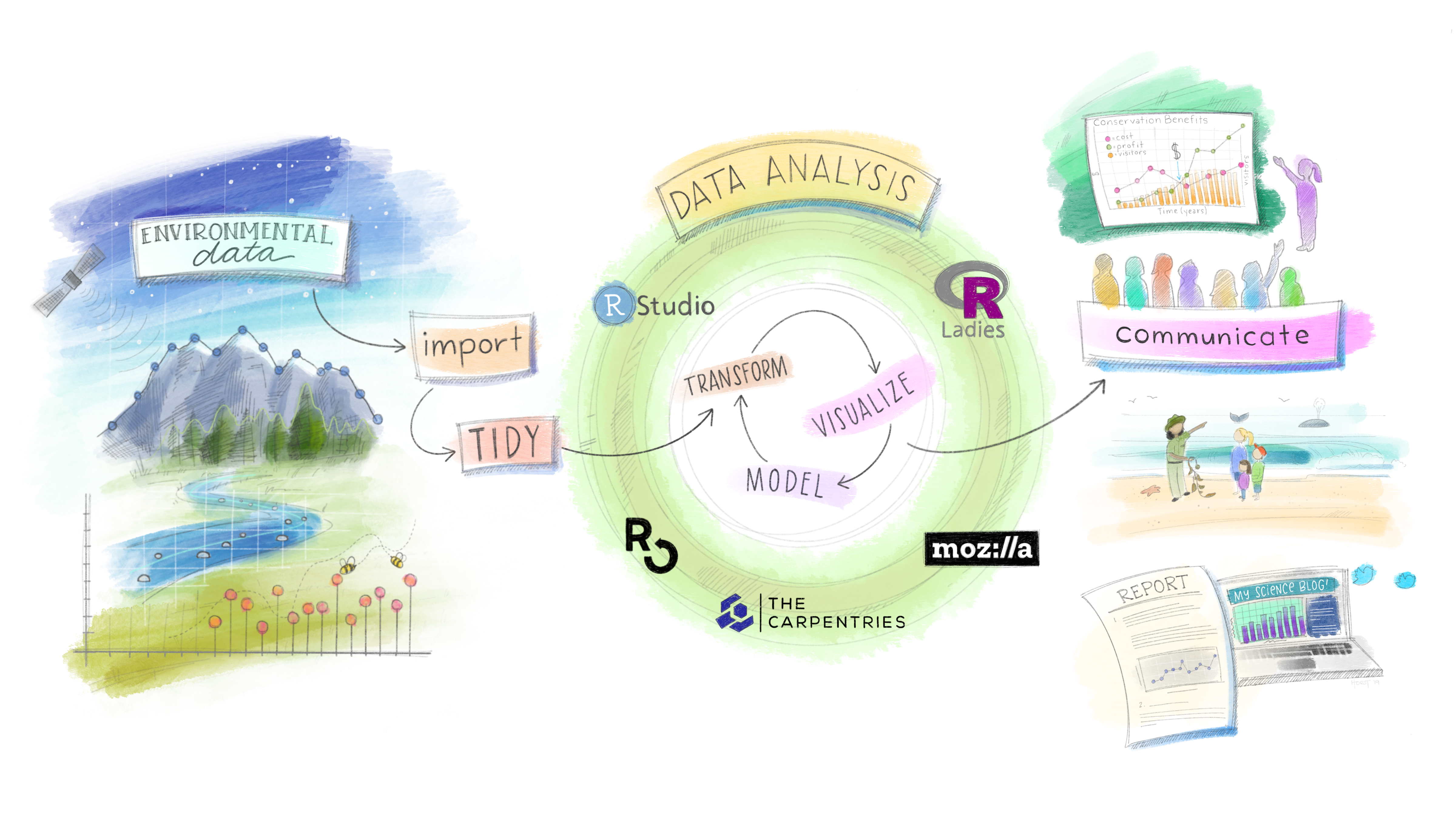
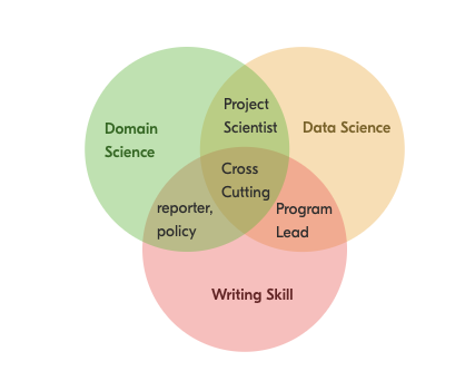
The Environmental Trifecta

Most environmental scientists have one or two of these. Few have all three.

Combining writing, data analysis, and domain expertise creates a rare and flexible professional — one who can move between science, policy, and practice.

AI can generate code. It cannot ask the right scientific question, evaluate whether the answer makes physical sense, or stand in front of a stakeholder and defend it. That combination is what we’re building.

“If not you, then who?”

Course Logistics

Instructor: Mike Johnson

Chief Data Scientist, Lynker
PhD in Geography, UC Santa Barbara
10+ years in hydrology and ecosystem science
Active work with NOAA, USACE, and federal water programs

The work we do in this course is in many ways the same work being done at the federal/state level right now. You’re learning a living skillset.

Course site:
https://mikejohnson51.github.io/csu-ess-523c/

Course Structure

Week	Topic
Week 1	Data Science Tools & Digital Environment
Week 2–3	Vector Data
Week 4	Raster Data
Week 5–6	Machine Learning
Week 7	Time Series

Grading

Setup 50 points - Due Wednesday — ensures your environment is ready for the course

Labs (6 × 150 pts = 900 pts)

Assigned Wednesdays, due the following Wednesday before class
All submissions via GitHub — version control is part of the grade
An optional final project (+150 pts extra credit) builds on your personal site from ESS 523a

Total: 950 pts (1100 possible with EC)

Grade Scale:

Grade	Range
A+	≥ 96.67%
A	93.33–96.67%
A–	90.0–93.33%
B+	86.67–90.0%
B	83.33–86.67%
B–	80.0–83.33%
C+	76.67–80.0%
C	70.0–76.67%
D	60.0–70.0%
F	< 60%

Working Together & AI Policy

Tip

Collaboration — encouraged

Discuss problems, share approaches, and help each other debug — you learn more working with peers.

Important

Individual work — required

Your code, writing, and results must be submitted individually.

Note

AI tools (ChatGPT, Claude, Copilot)

Acceptable: exploring concepts, debugging syntax, understanding errors, and short illustrative examples — always verify and understand outputs.
Not acceptable: producing final analyses, lab write-ups, figures, or any submission you present as solely your own work.
Disclosure: If AI contributed substantively, include a brief note describing the tool, model, and a short prompt summary.

Compute Needs

Your own computer running a full OS — Windows, macOS, or Linux
Chromebooks are not supported
If this is a barrier, reach out immediately and we’ll find a solution

Quantitative Reasoning

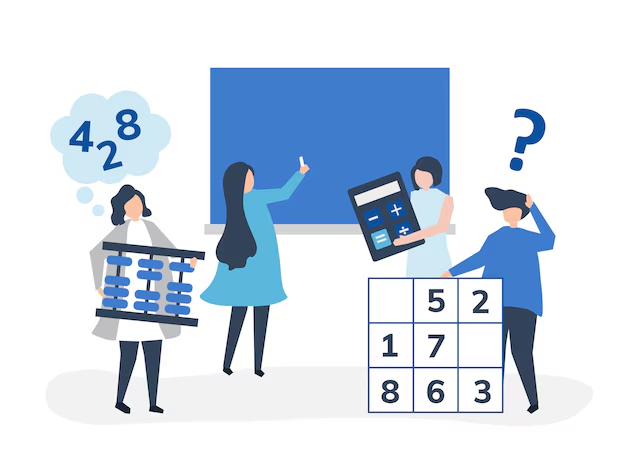
What Is Quantitative Reasoning?

Working Definition: Thinking about data from our world to better understand and make choices about the past, present, and future.

Many people can work with data (data scientists)
Many people have domain knowledge (hydrologists)
Few can do both carefully — that’s what makes you valuable

The rest of today is about building the foundation for that focusing on how computers store, find, and interpret information — and why that matters for doing science well.

Every Analysis Is a File Problem

Every piece of work in this course — and in your career — follows this chain:

Raw Data          ← files on disk, often from URLs or APIs
  ↓ R Scripts     ← read, clean, transform
Processed Data    ← files on disk
  ↓ R Scripts     ← model, summarize, visualize  
Outputs           ← figures, tables, reports — files on disk

A broken link anywhere in this chain means the analysis cannot be reproduced.

A file you can’t find, a path that only works on your machine, a format no one else can open — these are not minor inconveniences. They are scientific failures.

“An analysis is only as reproducible as the data you can find next year.”

Your Digital Environment

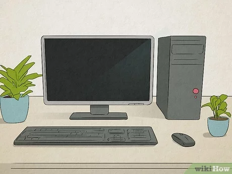
The Computer

Three subsystems you need to understand:

Disk: Persistent storage — files live here when the power is off. Reading from disk is slow.
Memory (RAM): Ephemeral workspace — data lives here while R runs. Fast, but finite and temporary.
CPU: Executes instructions — does the computation.

Why this matters for you:
When you load a 4 GB raster into R, it moves from disk into RAM. If your RAM is full, R crashes or slows to a crawl. Knowing where the bottleneck is (I/O? memory? compute?) is how you diagnose and fix slow analyses.

The Compute Cycle

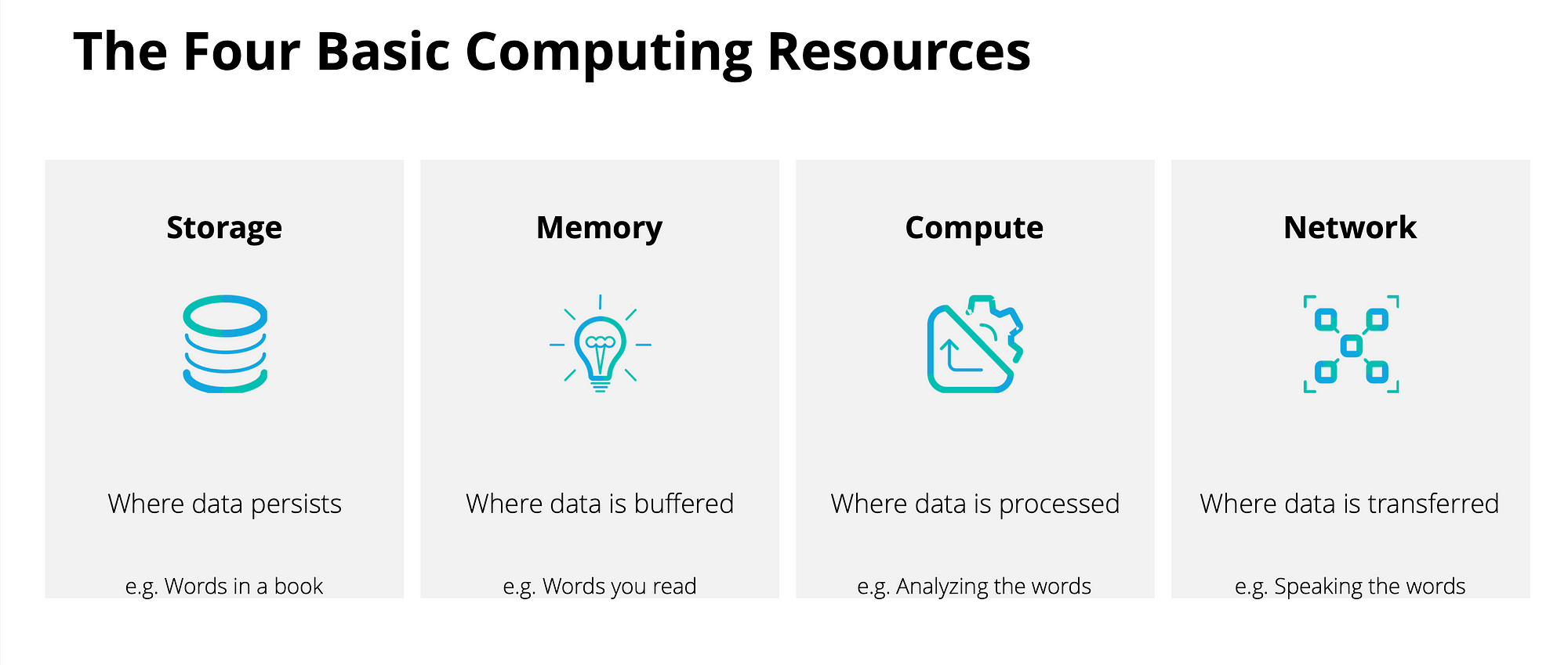
Data flows: disk → memory → CPU → memory → disk

Every read_csv(), st_read(), and rast() call you make starts this cycle. Every write_csv() and writeRaster() ends it.

Bytes

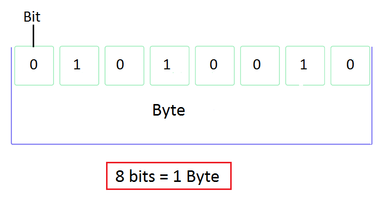
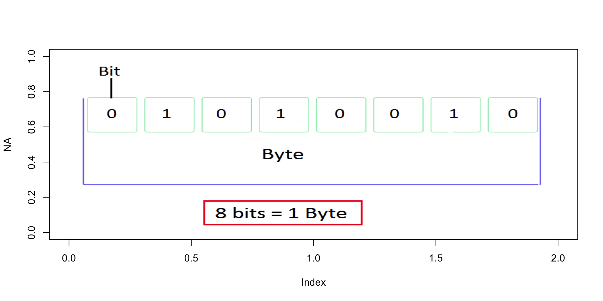
Bits and Bytes

A bit is one logical state: 0 or 1
A byte is 8 bits
Everything on a computer — text, images, spatial data, model outputs — is bytes

Why it matters in practice:

Dataset	Size estimate
USGS daily flow record, 1 gauge, 50 years	~150 KB
NHDPlus HR flowlines, CONUS	~12 GB
NWM retrospective, 1 variable, 1 year	~200 GB
3DEP 1m DEM, single HUC4	~8–40 GB

These numbers stop being surprising once you know the unit chain: KB → MB → GB → TB (each ×1,024).

Files

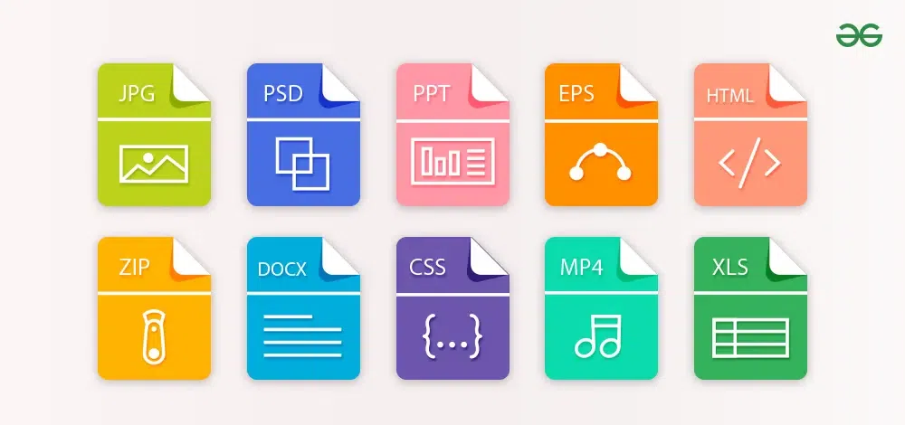
What Is a File?

Files save bytes on disk in a structured, meaningful way
Every file has three key properties:
- A name — how you and the computer identify it
- A path — its address in the file system hierarchy
- An extension — tells programs how to interpret the bytes
Hard drives don’t understand files — they store bytes. The file system is the organizational layer that makes bytes into named, navigable objects.

File Systems & Directories

How operating systems differ:

Windows : drives (C:\), backslash separators
macOS / Linux : forward slashes, everything under root /
Cloud (S3, GCS): looks like a filesystem, but is actually flat key-value storage

Key vocabulary:

Term	Meaning
Root	Top-level directory — contains everything
Working directory	Where your session is (`getwd()`)
Parent directory	One level up (`..`)
Subdirectory	A folder inside the working directory

File Naming

The Importance of Names

Tip

“There are only two hard things in Computer Science: cache invalidation and naming things.” ~Phil Karlton

File names are how you — and your collaborators — navigate a project. There is no enforced standard. The decisions are always yours.

Bad names compound silently. One bad name is annoying. A project full of them is a crisis.

Three Principles

Machine readable — unambiguous, parseable, regex-friendly
Human readable — tells you what’s inside without opening it
Sortable — natural order reflects logical order

Machine Readable

No spaces, no punctuation, no accented characters, no mixed case
Use regular expression friendly (e.g. use patterns!)
Use ISO 8601 dates: YYYY-MM-DD — they sort correctly as strings
Consistent delimiters:
- _ separates metadata fields
- - separates words within a field

This makes files easy to …

Search Programmatically:

files <- list.files("data/usgs-files", pattern = "_tx")
length(files)
#> [1] 27

#> [1] "1903-07-01_08033500_00060_tyler_tx.txt"   
#> [2] "1923-10-01_08033000_00060_angelina_tx.txt"

Operate on:

Metadata is recoverable without opening a single file:

stringr::str_split(files, "[_\\.]", simplify = TRUE)

#>    StartDate   siteID parameterCode   county state extension
#> 1 1903-07-01 08033500         00060    tyler    tx       txt
#> 2 1923-10-01 08033000         00060 angelina    tx       txt
#> 3 1923-10-01 08180500         00060   medina    tx       txt
#> 4 1923-12-01 08082500         00060   baylor    tx       txt
#> 5 1924-08-01 08062500         00060    ellis    tx       txt

Human Readable + Sortable

Human readable — the name communicates content and purpose. Here, we see the order that the files run (utilities, download, clean, analyze, figures), the project they belong to (src), are archived in the file names.

list.files("R")
#> [1] "00_src_utils.R"         "01_src_data-download.R" "02_src_data-clean.R"   
#> [4] "03_src_analysis.R"      "04_src_figures.R"

#>   Order Project       Purpose extension
#> 1    00     src         utils         R
#> 2    01     src data-download         R
#> 3    02     src    data-clean         R
#> 4    03     src      analysis         R
#> 5    04     src       figures         R

Sortable — leading zeros and ISO dates keep files in logical order:

✅  01_src_download.R       2024-01-15_sw-discharge_co.csv
    02_src_clean.R          2024-02-03_sw-discharge_co.csv
    03_src_analyze.R        2024-11-20_sw-discharge_co.csv

❌  1_download.R            01-15-2024_data.csv
    10_figures.R            11-20-2024_data.csv
    2_clean.R               02-03-2024_data.csv

File Paths

System of Directions

File paths tell us the location of a file within the file system
Directories are stored as hierarchies, again with root (home) directory being the one holding everything on a system
The folder you are in, is called your working directory. (think pwd)
The folder above the working directory is the parent directory
All folders within the working directory are sub folders or child folder

Absolute vs. Relative Paths

Absolute — starts from root, always resolves, but only on your machine:

img <- png::readPNG('/Users/mikejohnson/github/csu-523c-2026/slides/img/03-bit-byte.png')

Relative — starts from the working directory, works anywhere the project is opened:

img <- png::readPNG('img/03-bit-byte.png')

. and .. shorthand:

.    = this directory
..   = the parent directory

../data/raw/flow.csv   →  up one level, then into data/raw/

Important

Absolute paths are the #1 reproducibility killer in shared projects. If your code contains /Users/yourname/, it will break the moment anyone else runs it — including future you on a new machine.

RStudio Projects + `here`

Tip

RStudio Projects (.Rproj) automatically set the working directory to the project root when opened — making relative paths reliable by default.

Best practices:

Keep all project files together: raw data, scripts, outputs, figures
Never hardcode paths outside the project root
Use here::here() for paths inside packages or Quarto documents — it anchors to the project root regardless of where the .qmd lives

# Always resolves from project root, never from the .qmd file's location
here::here("data", "raw", "flow_2024.csv")
#> /Users/mikejohnson/github/csu-523c-2026/data/raw/flow_2024.csv

Enforcing Relative Paths

Tip

Working with absolute paths can be a pain compared to relative paths…

It is a good practice to keep all the files associated with a project — input data, R scripts, analytic results, figures - together.
This is such a common practice that RStudio has built-in support for this via projects.
A good project layout will ultimately make your life easier:
- It will help ensure the integrity of your data;
- It makes it simpler to share your code with someone else (a lab-mate, collaborator, or supervisor);
- It allows you to easily upload your code with your manuscript submission;
- It makes it easier to pick the project back up after a break.

File Extensions

Context

All files store bits.
Extensions can be considered a type of metadata that provides information about the way data might be stored
There are 1000’s of different formats for data ranging from common to custom
Each format defines how the sequence of bits and bytes are laid out
Indicate the characteristics of the file, its intended use, and the default applications that can open/use the file.
If you double click a .docx file it opens in Word which interprets the meaning of the bytes
If you double click an .R file it opens with RStudio, and R interprets the meaning of the bytes

Extension Interpretation

Readers depended on anticipated structure

img <- jpeg::readJPEG('img/03-bit-byte.png')
#> Error in jpeg::readJPEG("img/03-bit-byte.png"): JPEG decompression error: Not a JPEG file: starts with 0x89 0x50

The file is actually a PNG with the wrong file extension. “0x89 0x50” is how a PNG file starts.

img <- png::readPNG('img/03-bit-byte.png')

The data returned to R is a structured set of bits, interpreted according to the directions of the file and the interpreting language!

dim(img)
#> [1] 394 768   3
class(img)
#> [1] "array"
str(img)
#>  num [1:394, 1:768, 1:3] 1 1 1 1 1 1 1 1 1 1 ...

Information pass through:

Bytes Being Interpreted

# Character Object
(x <- "CSU 523C")

#> [1] "CSU 523C"

Bytes Being Interpreted

# Character Object
(x <- "CSU 523C")

# Character Object to Raw Type
# How R sees the data
(y <- charToRaw(x))

#> [1] "CSU 523C"
#> [1] 43 53 55 20 35 32 33 43

Bytes Being Interpreted

# Character Object
(x <- "CSU 523C")

# Character Object to Raw Type
# How R sees the data
(y <- charToRaw(x))

# Raw to Bits
# Whats on disk
(z <- rawToBits(y))

#> [1] "CSU 523C"
#> [1] 43 53 55 20 35 32 33 43
#>  [1] 01 01 00 00 00 00 01 00 01 01 00 00 01 00 01 00 01 00 01 00 01 00 01 00 00
#> [26] 00 00 00 00 01 00 00 01 00 01 00 01 01 00 00 00 01 00 00 01 01 00 00 01 01
#> [51] 00 00 01 01 00 00 01 01 00 00 00 00 01 00

Bytes Being Interpreted

# Character Object
(x <- "CSU 523C")

# Character Object to Raw Type
# How R sees the data
(y <- charToRaw(x))

# Raw to Bits
# Whats on disk
(z <- rawToBits(y))

length(z)

#> [1] "CSU 523C"
#> [1] 43 53 55 20 35 32 33 43
#>  [1] 01 01 00 00 00 00 01 00 01 01 00 00 01 00 01 00 01 00 01 00 01 00 01 00 00
#> [26] 00 00 00 00 01 00 00 01 00 01 00 01 01 00 00 00 01 00 00 01 01 00 00 01 01
#> [51] 00 00 01 01 00 00 01 01 00 00 00 00 01 00
#> [1] 64

Bytes Being Interpreted

# Character Object
(x <- "CSU 523C")

# Character Object to Raw Type
# How R sees the data
(y <- charToRaw(x))

# Raw to Bits
# Whats on disk
(z <- rawToBits(y))

length(z)

nchar(x)

#> [1] "CSU 523C"
#> [1] 43 53 55 20 35 32 33 43
#>  [1] 01 01 00 00 00 00 01 00 01 01 00 00 01 00 01 00 01 00 01 00 01 00 01 00 00
#> [26] 00 00 00 00 01 00 00 01 00 01 00 01 01 00 00 00 01 00 00 01 01 00 00 01 01
#> [51] 00 00 01 01 00 00 01 01 00 00 00 00 01 00
#> [1] 64
#> [1] 8

Bytes Being Interpreted

# Character Object
(x <- "CSU 523C")

# Character Object to Raw Type
# How R sees the data
(y <- charToRaw(x))

# Raw to Bits
# Whats on disk
(z <- rawToBits(y))

length(z)

nchar(x)

nchar(x) == (length(z)/8)

#> [1] "CSU 523C"
#> [1] 43 53 55 20 35 32 33 43
#>  [1] 01 01 00 00 00 00 01 00 01 01 00 00 01 00 01 00 01 00 01 00 01 00 01 00 00
#> [26] 00 00 00 00 01 00 00 01 00 01 00 01 01 00 00 00 01 00 00 01 01 00 00 01 01
#> [51] 00 00 01 01 00 00 01 01 00 00 00 00 01 00
#> [1] 64
#> [1] 8
#> [1] TRUE

How images are rendered:

plot(NA, xlim = c(0, 2), ylim = c(0, 1))
rasterImage(img, 0, 0, 2, 1)

Common Formats in Water Resources Data Science

Format	Type	Common Use
`.csv`	Text	Tabular field data, gauge records, water quality
`.json` / `.geojson`	Structured	Web APIs, geographic feature exchange
`.tif` / `.geotiff`	Binary	Satellite imagery, DEMs, classified rasters
`.nc` (NetCDF)	Binary	NWM output, climate models, multi-dimensional arrays
`.gpkg` (GeoPackage)	Structured	Vector + raster, open standard, replaces Shapefile
`.shp` (Shapefile)	Binary	Legacy vector data — still everywhere, many limitations
`.parquet`	Binary	Large tabular/spatial data, fast I/O, cloud-native

URLs as File Paths

URL Structure

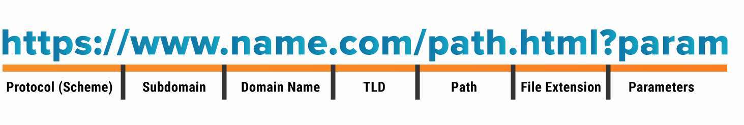
Part	Example	Analogy
Protocol	`https://`, `s3://`	How to travel
Domain	`waterservices.usgs.gov`	The server (building)
Path	`/nwis/iv/`	Directory (floor/room)
File	`flow_2024.csv`	The file
Parameters	`?sites=06752260&parameterCd=00060`	Filters on the request

URLs Are Just Remote Paths

The file system logic you just learned applies directly to URLs:

https://mikejohnson51.github.io/csu-ess-330/slides/1-welcome.html#/title-slide
         ↑ server (domain)      ↑ directory   ↑ file             ↑ anchor

s3://noaa-nwm-retrospective-3-0-pds/CONUS/zarr/chrtout.zarr
     ↑ bucket                        ↑ directory  ↑ file

And URLs are your data pipeline:

# USGS streamflow — the path IS the query
url <- "https://waterservices.usgs.gov/nwis/iv/?sites=06752260&parameterCd=00060&format=json"
data <- jsonlite::fromJSON(url)

dplyr::glimpse(data)(data)

# NWM retrospective on S3 — same concept, different protocol
s3_path <- "s3://noaa-nwm-retrospective-3-0-pds/CONUS/zarr/chrtout.zarr"

Query parameters (?sites=...&parameterCd=...) filter data at the server before it reaches your machine. Understanding URL structure means understanding how to ask for exactly what you need.

Putting It Together

Every analysis: question → data (files + paths + formats) → compute → output (files + paths + formats)

The concepts from today — bytes, files, names, paths, extensions, URLs — are the substrate every analysis runs on. They feel like setup. They are actually the foundation.

5-Minute Break

Take five — stretch, hydrate, and reset.

Return in 5 minutes.

R + RStudio

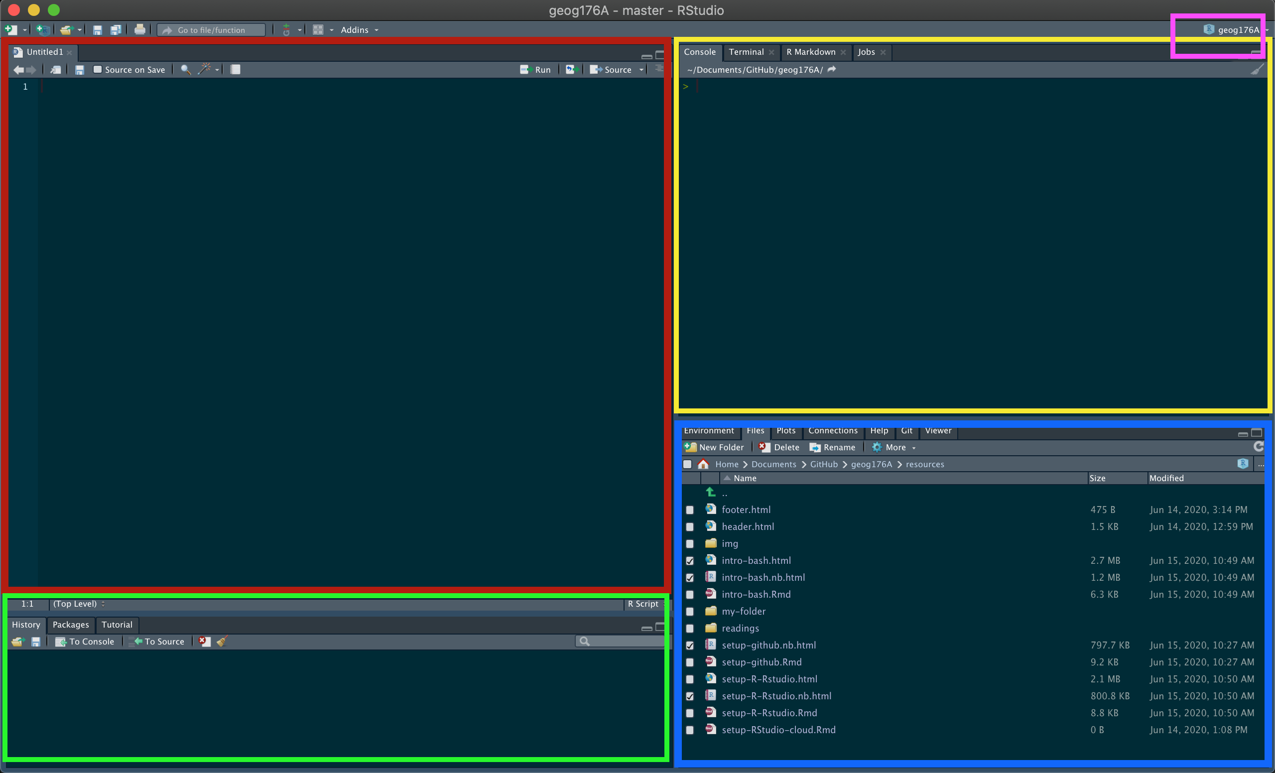
R vs. RStudio

These are two separate things. Confusing them is the most common source of early frustration.

R — the language and engine - Does the actual computation - Runs without RStudio - Must be installed first

RStudio — the IDE (development environment) - The interface you’ll look at all day - Organizes files, environment, plots, packages, terminal - Makes R usable — but it is not R

Analogy: R is the engine. RStudio is the dashboard and steering wheel. You need both, but they are not the same thing.

The Four Panes

Pane	Location	Purpose
Source	Top left	Write and save scripts — your permanent work
Console / Terminal	Top right	Run R interactively; access the shell
History / Packages / Git	Bottom left	Command history, package manager, version control
Environment / Files / Plots / Help	Bottom right	Objects in memory, file browser, output viewer, documentation

Important

The console does not save your work. Anything you run there and don’t put in a script is gone when you close RStudio. Build the habit early: if it matters, it goes in a script.

Packages: Extending R

Base R: ships with R — vectors, data frames, basic statistics, plots
Packages: functions written by the community, installed from CRAN (or github/biocondutor/etc), loaded per session

install.packages("sf")   # once per machine
library(sf)              # once per session

Core packages for this course:

Package	Purpose
`tidyverse`	Data manipulation (`dplyr`, `tidyr`) and visualization (`ggplot2`)
`sf`	Vector spatial data — points, lines, polygons
`terra`	Raster spatial data — grids, DEMs, satellite imagery
`tidymodels`	Machine learning with tidy principles

Version Control

You Have Already Done This

analysis_final.R
analysis_final_v2.R
analysis_final_ACTUAL_FINAL.R
analysis_mikereview_jan12.R
analysis_mikereview_jan12_USETHISONE.R

This is version control, just done badly.

It doesn’t tell you what changed, why it changed, or which version to trust. It breaks completely the moment two people work on the same file.

Git provides a solution.
It tracks every change to every file — with a timestamp, an author, and a message — and lets you revert to any previous state. Not just for code: data, reports, quarto documents, everything.

Git + GitHub

Git runs on your machine — the version control engine

GitHub hosts your repositories in the cloud — collaboration, backup, and portfolio in one place

Together:

Complete, auditable history of every project
Collaborate without overwriting each other
Revert any file to any previous state
Public portfolio of your work
The standard for open, reproducible science

All labs in this course are submitted via GitHub. We set it up together in this week’s homework — by next class, this will already be part of your workflow.

The Terminal

Your Power Tool

The terminal is a text interface to your file system. It feels archaic. It is indispensable.

Git, package installation, server connections, working in the cloud — all of it eventually touches the terminal. The sooner it feels normal, the better.

Command	Does
`pwd`	Where am I?
`ls`	What’s here?
`cd folder`	Move into `folder`
`cd ..`	Move up one level
`mkdir name`	Create a directory name
`cp a b`	Copy `a` to `b`
`mv a b`	Move / rename `a` to `b`

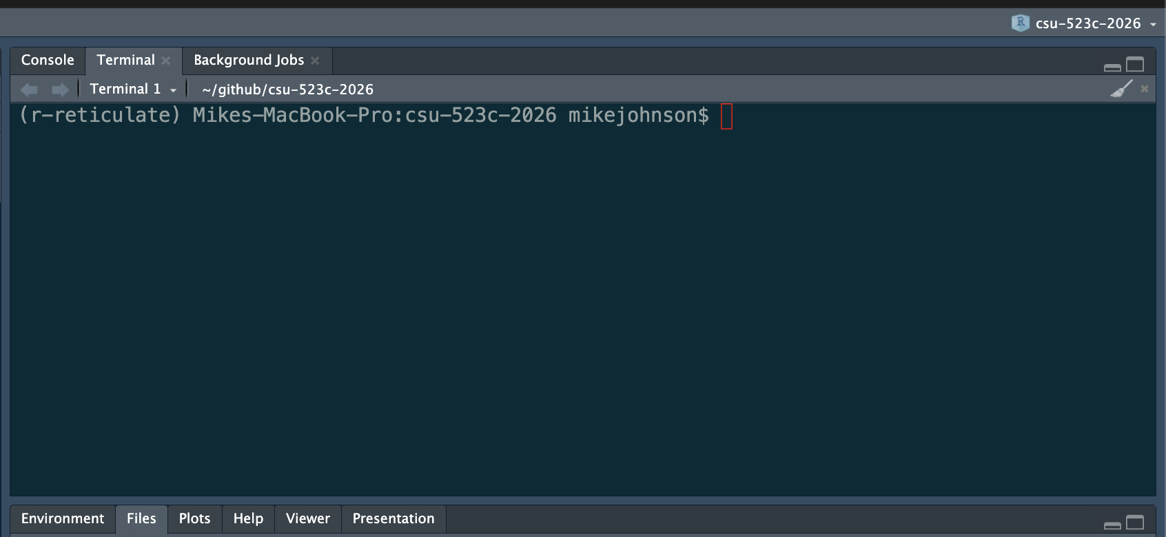
In RStudio: Terminal tab, next to Console — use it there until the standalone terminal feels comfortable.

Before Next Class

This week’s homework ensures your environment is ready:

Lab 00: Verify Your Environment + Meet Your Tools
Confirm your R, RStudio, and Git setup — install course packages, configure Git, connect to GitHub. Come to the next class ready to code!

Next topic: Data Manipulation crash course

Week 1

Agenda & Timing

Today’s flow (1 hr 50 min)

Welcome

What This Class Is About

The Environmental Trifecta

Course Logistics

Instructor: Mike Johnson

Course Structure

Grading

Working Together & AI Policy

Compute Needs

Quantitative Reasoning

What Is Quantitative Reasoning?

Every Analysis Is a File Problem

Your Digital Environment

The Computer

The Compute Cycle

Bytes

Bits and Bytes

Files

What Is a File?

File Systems & Directories

File Naming

The Importance of Names

Three Principles

Machine Readable

Search Programmatically:

Operate on:

Human Readable + Sortable

File Paths

System of Directions

Absolute vs. Relative Paths

RStudio Projects + here

Enforcing Relative Paths

File Extensions

Context

Extension Interpretation

Information pass through:

Bytes Being Interpreted

Bytes Being Interpreted

Bytes Being Interpreted

Bytes Being Interpreted

Bytes Being Interpreted

Bytes Being Interpreted

How images are rendered:

Common Formats in Water Resources Data Science

URLs as File Paths

URL Structure

URLs Are Just Remote Paths

Putting It Together

5-Minute Break

Take five — stretch, hydrate, and reset.

R + RStudio

R vs. RStudio

The Four Panes

Packages: Extending R

Version Control

You Have Already Done This

Git + GitHub

The Terminal

Your Power Tool

Before Next Class

This week’s homework ensures your environment is ready:

Next topic: Data Manipulation crash course

RStudio Projects + `here`