#> [1] 31254Week 3
Predicates, Simplification & Tesselations
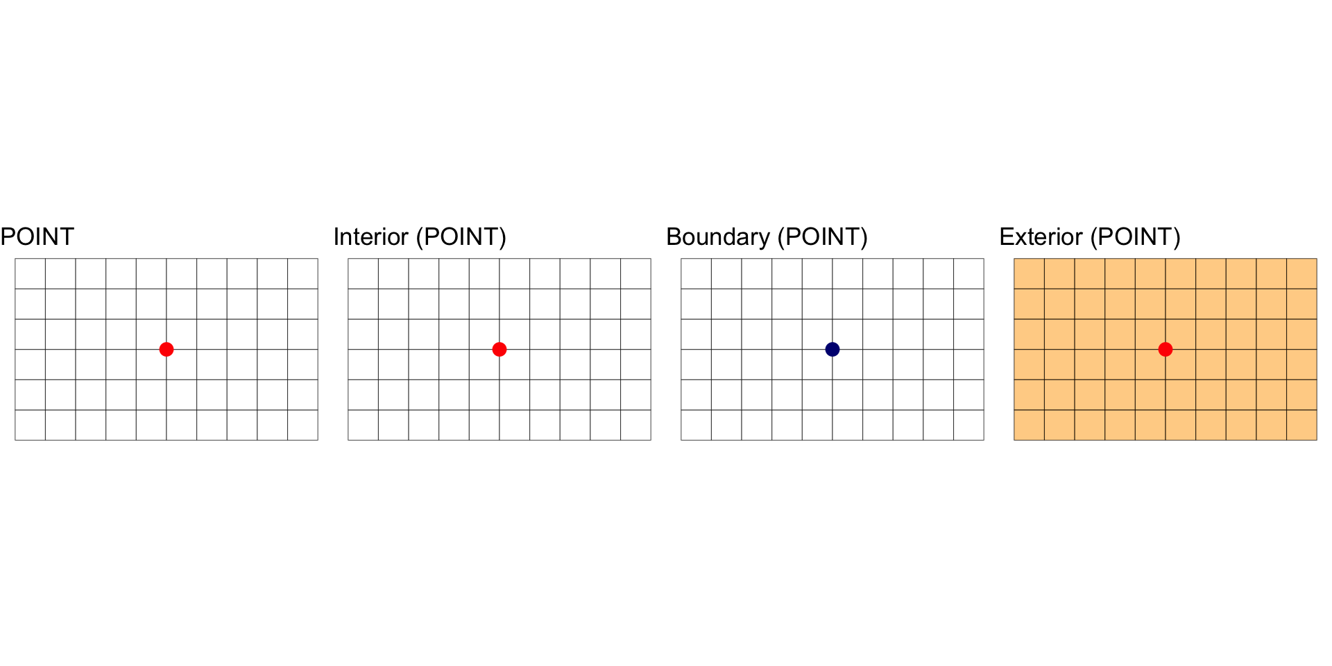
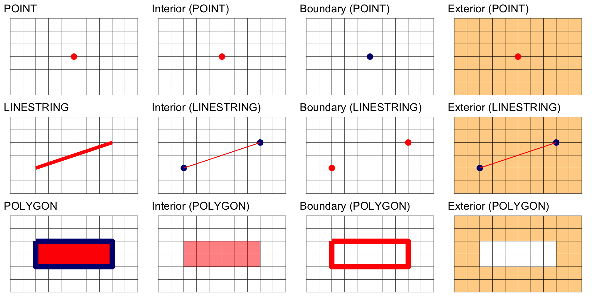
Interior, Boundary and Exterior: POINTS
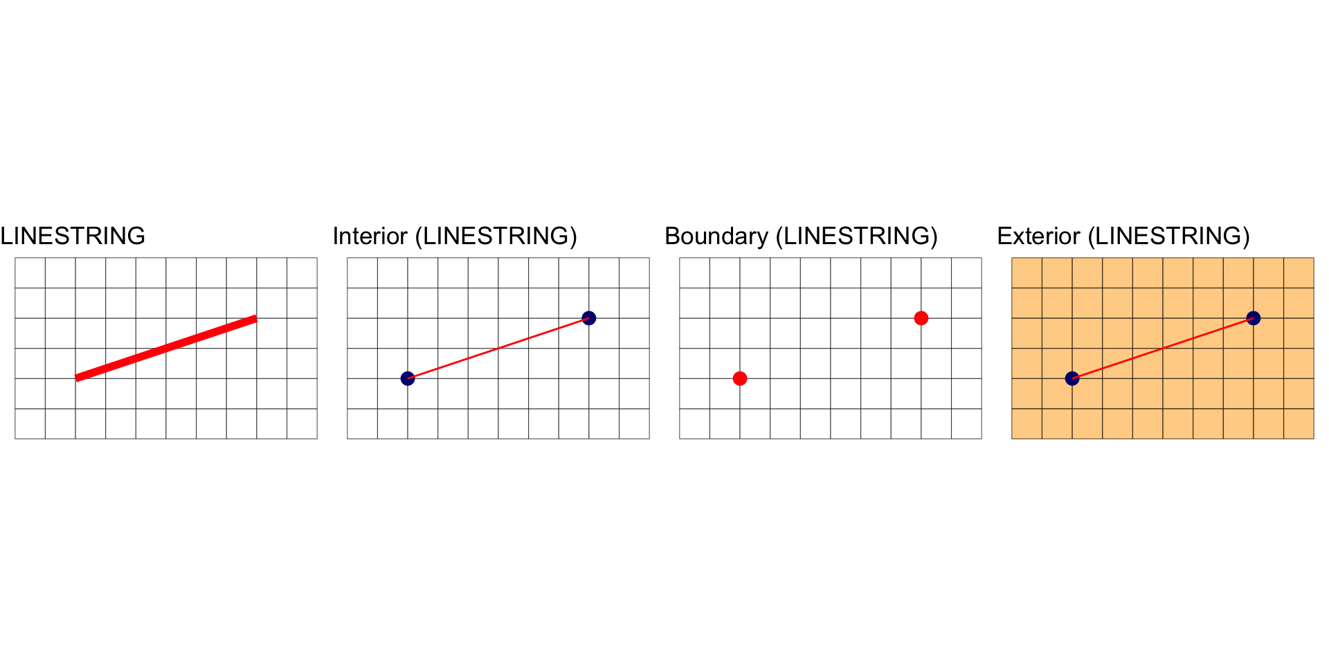
Interior, Boundary and Exterior: LINESTRING
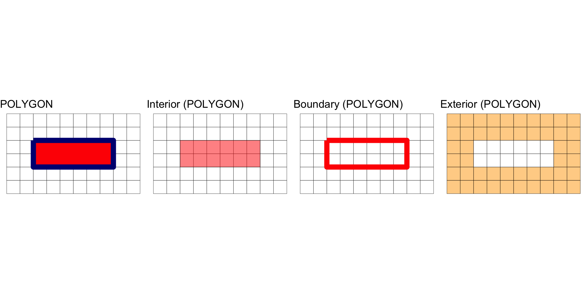
Interior, Boundary and Exterior: POLYGON
Summary
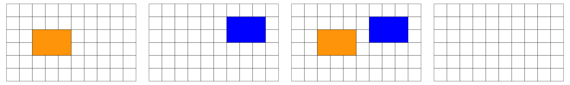
Overlap is a POINT: 0D
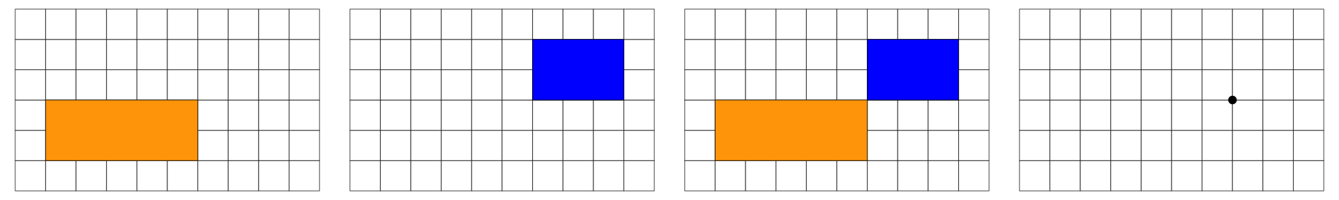
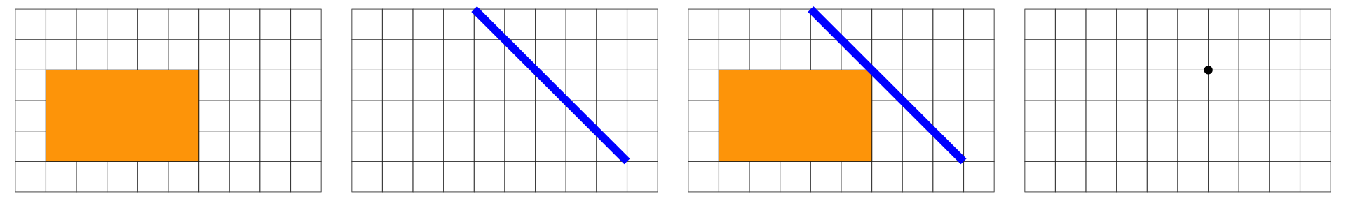
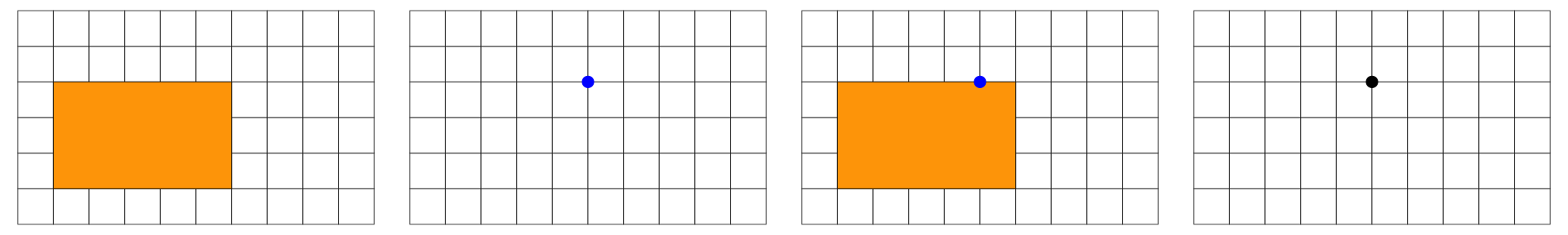
Overlap is a LINESTRING: 1D
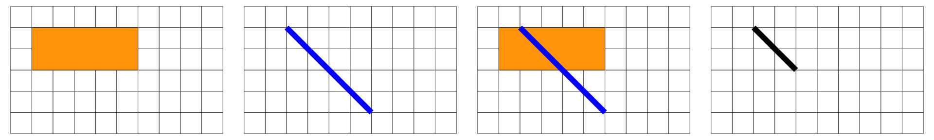
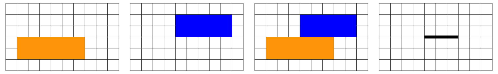
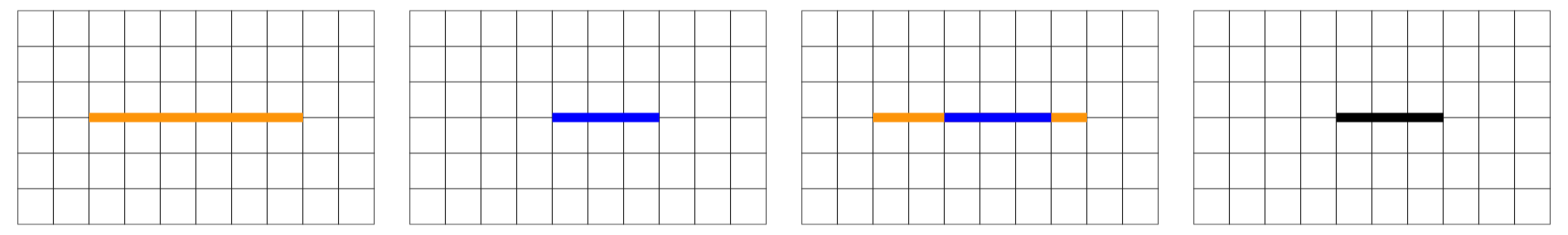
Overlap is a POLYGON: 2D
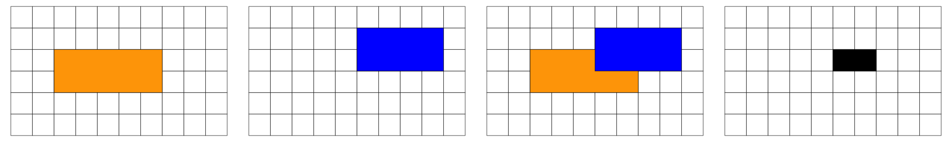
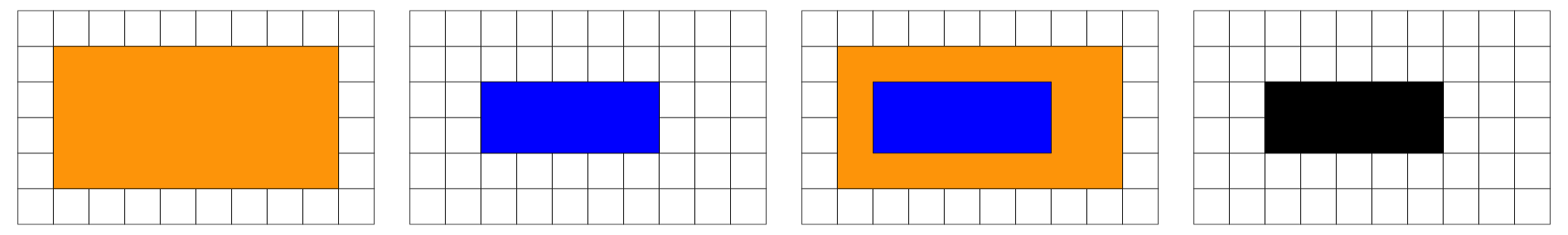
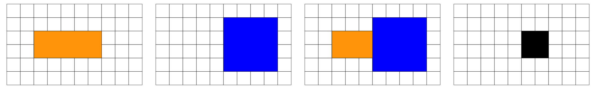
No Overlap = FALSE
The Matrix Model
The DE-9IM matrix is based on a 3x3 intersection matrix:
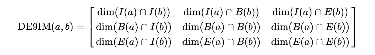
Where:
- dim is the dimension of the intersection and
- I is the interior
- B is the boundary
- E is the exterior
Empty sets are denoted as F
non-empty sets are denoted with the maximum dimension of the intersection {0,1,2}
A simpler (binary) version of this matrix can be created by mapping all non-empty intersections {0,1,2} to TRUE.

Where II would state: “Does the Interior of”a” overlaps with the Interior of “b” in a way that produces a point (0), line (1), or polygon (2)”
Where IB would state: “Does the Interior of”a” overlap with the Boundary of “b” in a way that produces a point (0), line (1), or polygon (2)”
Both matrix forms:
- dimensional {0,1,2,F}
- Boolean {T,F}
Can be serialize as a “DE-9IM string code” representing the matrix in a single string element (standardized format for data interchange)
The OGC has standardized the typical spatial predicates (Contains, Crosses, Intersects, Touches, etc.) as Boolean functions, and the DE-9IM model as a function that returns the DE-9IM code, with domain of {0,1,2,F}
Illustration
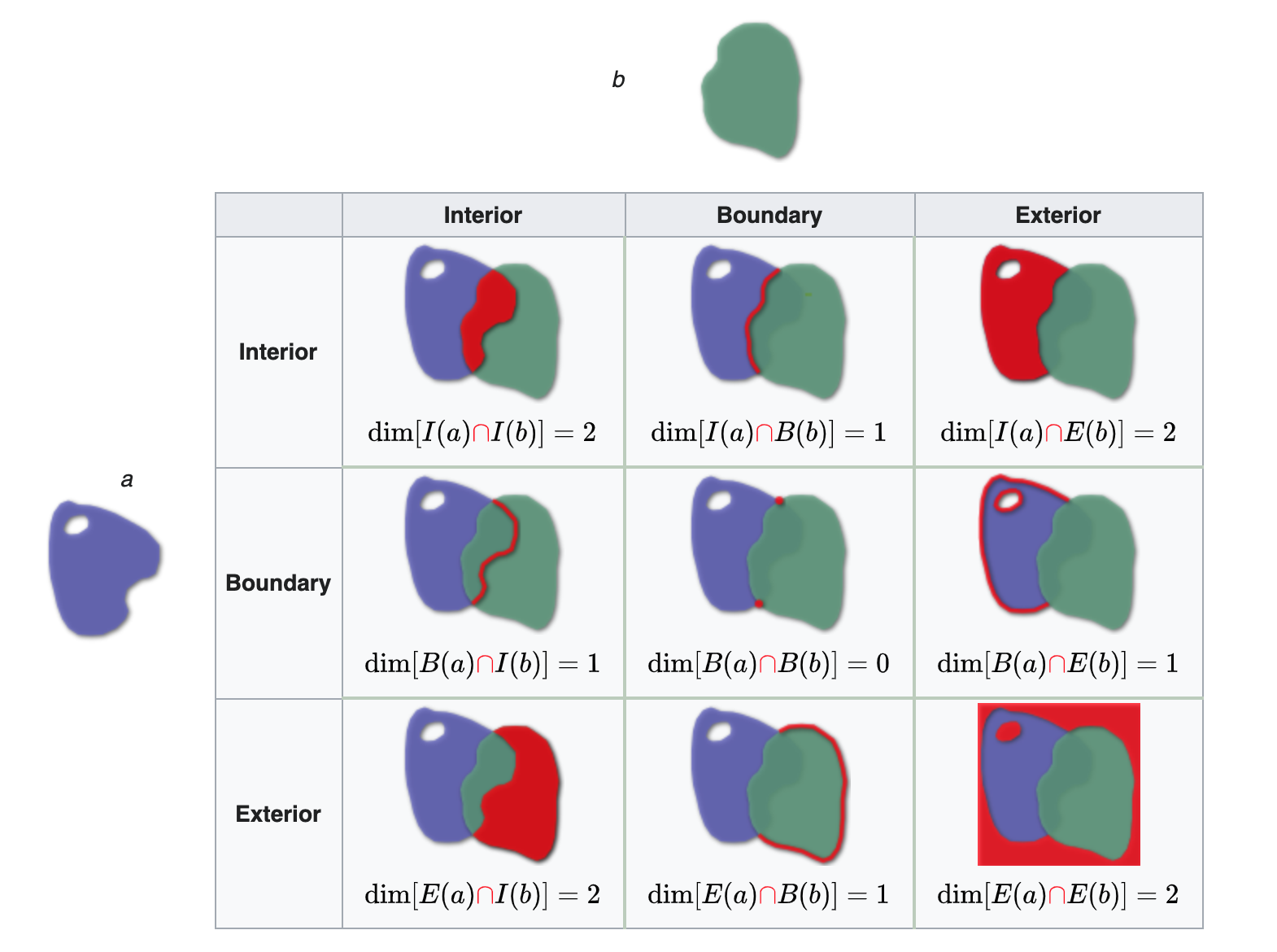
Reading from left-to-right and top-to-bottom, the DE-9IM(a,b) string code is ‘212101212’
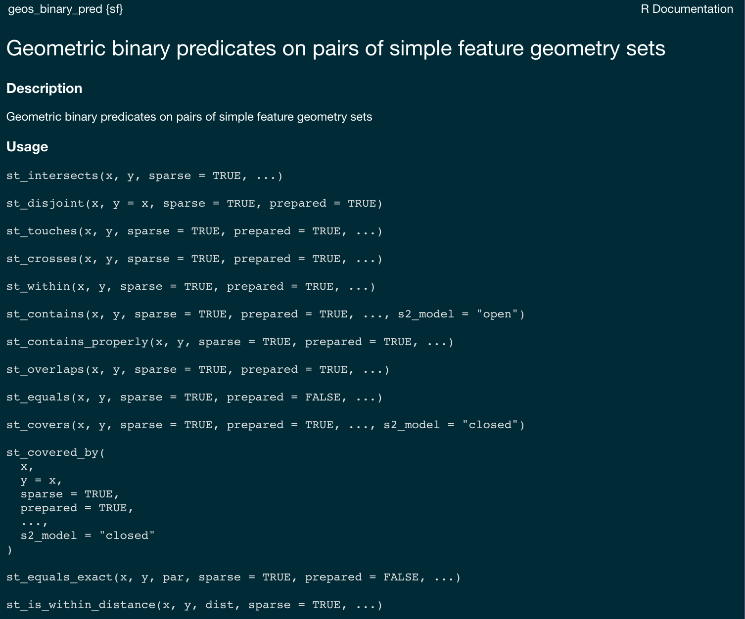
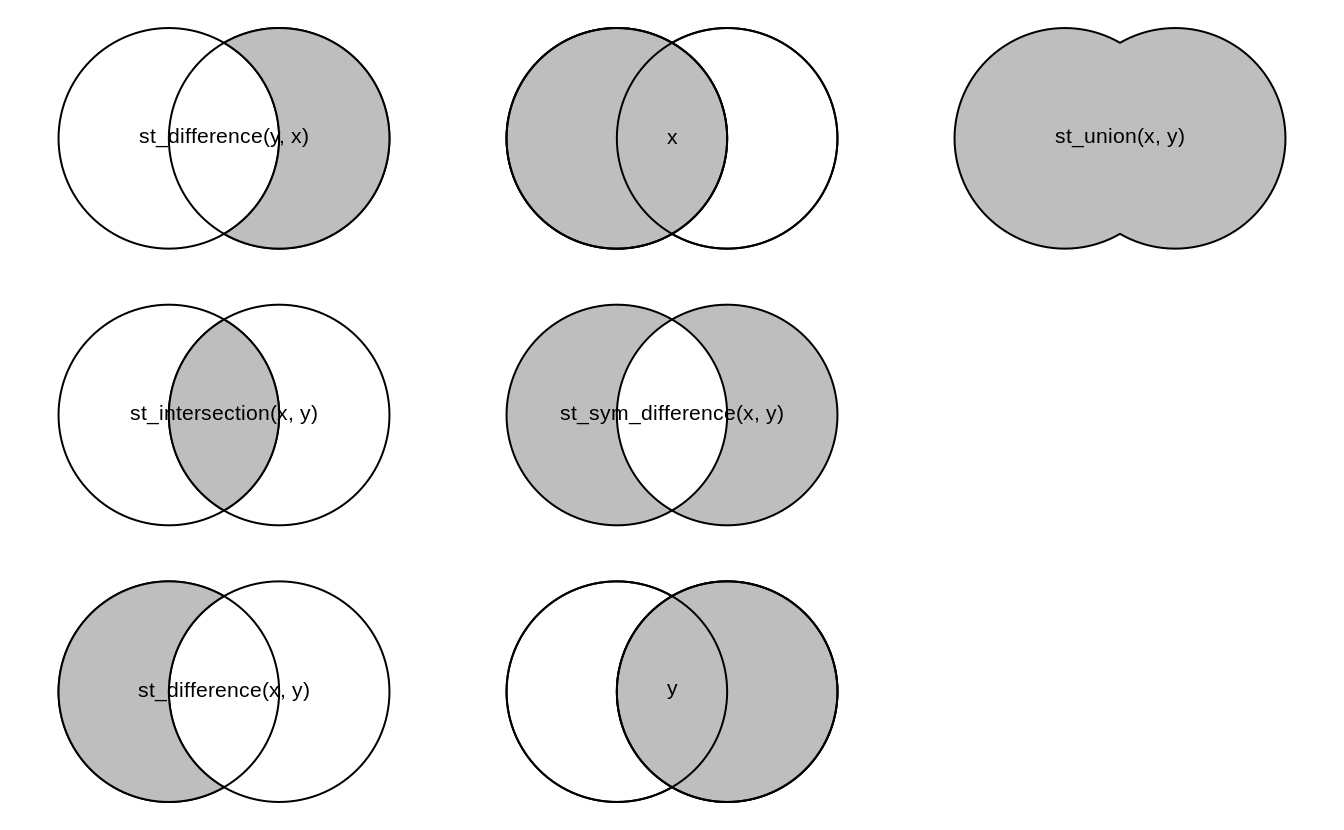
Spatial Relations in R
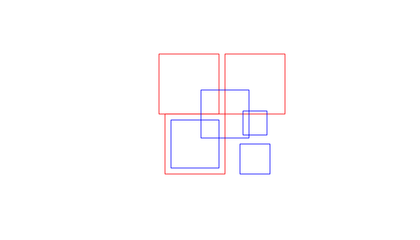
- Geometry X is a 3 feature polygon colored in red
- Geometry Y is a 4 feature polygon colored in blue
#>      [,1]        [,2]        [,3]        [,4]
#> [1,] "212FF1FF2" "FF2FF1212" "212101212" "FF2FF1212"
#> [2,] "FF2FF1212" "212101212" "212101212" "FF2FF1212"
#> [3,] "FF2FF1212" "FF2FF1212" "212101212" "FF2FF1212"
#>      [,1]        [,2]        [,3]
#> [1,] "2FFF1FFF2" "FF2F01212" "FF2F11212"
#> [2,] "FF2F01212" "2FFF1FFF2" "FF2FF1212"
#> [3,] "FF2F11212" "FF2FF1212" "2FFF1FFF2"
#>      [,1]        [,2]        [,3]        [,4]
#> [1,] "2FFF1FFF2" "FF2FF1212" "212101212" "FF2FF1212"
#> [2,] "FF2FF1212" "2FFF1FFF2" "212101212" "FF2FF1212"
#> [3,] "212101212" "212101212" "2FFF1FFF2" "FF2FF1212"
#> [4,] "FF2FF1212" "FF2FF1212" "FF2FF1212" "2FFF1FFF2"Binary Predicates
Collectively, predicates define the type of relationship each 2D object has with another.
Of the ~ 512 unique relationships offered by the DE-9IM models a selection of ~ 10 have been named.
These are included in PostGIS/GEOS and are made accessible via R sf
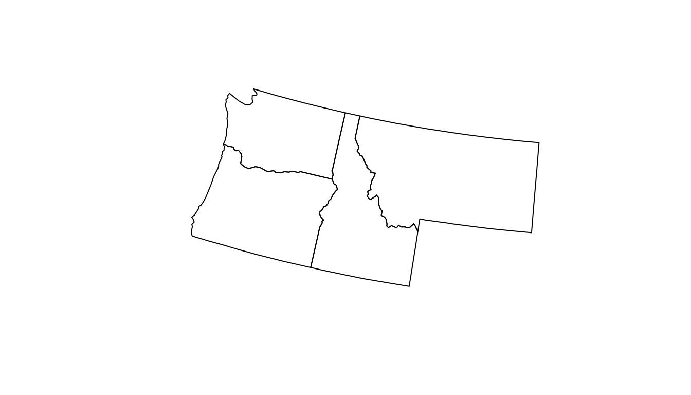
st_relates vs. predicate calls…
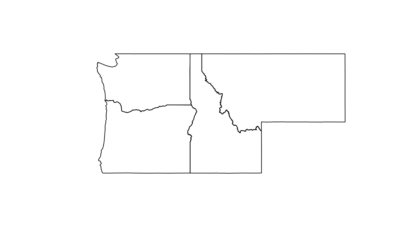
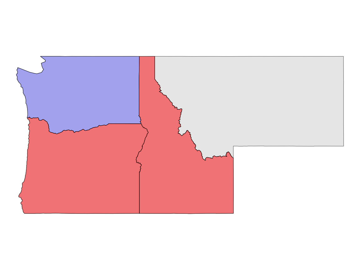
#> Simple feature collection with 4 features and 3 fields
#> Geometry type: MULTIPOLYGON
#> Dimension:     XY
#> Bounding box:  xmin: -124.8485 ymin: 41.98818 xmax: -104.0397 ymax: 49.00244
#> Geodetic CRS:  WGS 84
#>         name                       geometry     deim9 touch
#> 1      Idaho MULTIPOLYGON (((-111.0455 4... FF2F11212  TRUE
#> 2    Montana MULTIPOLYGON (((-109.7985 4... FF2FF1212 FALSE
#> 3     Oregon MULTIPOLYGON (((-117.22 44.... FF2F11212  TRUE
#> 4 Washington MULTIPOLYGON (((-121.5237 4... 2FFF1FFF2 FALSEResult
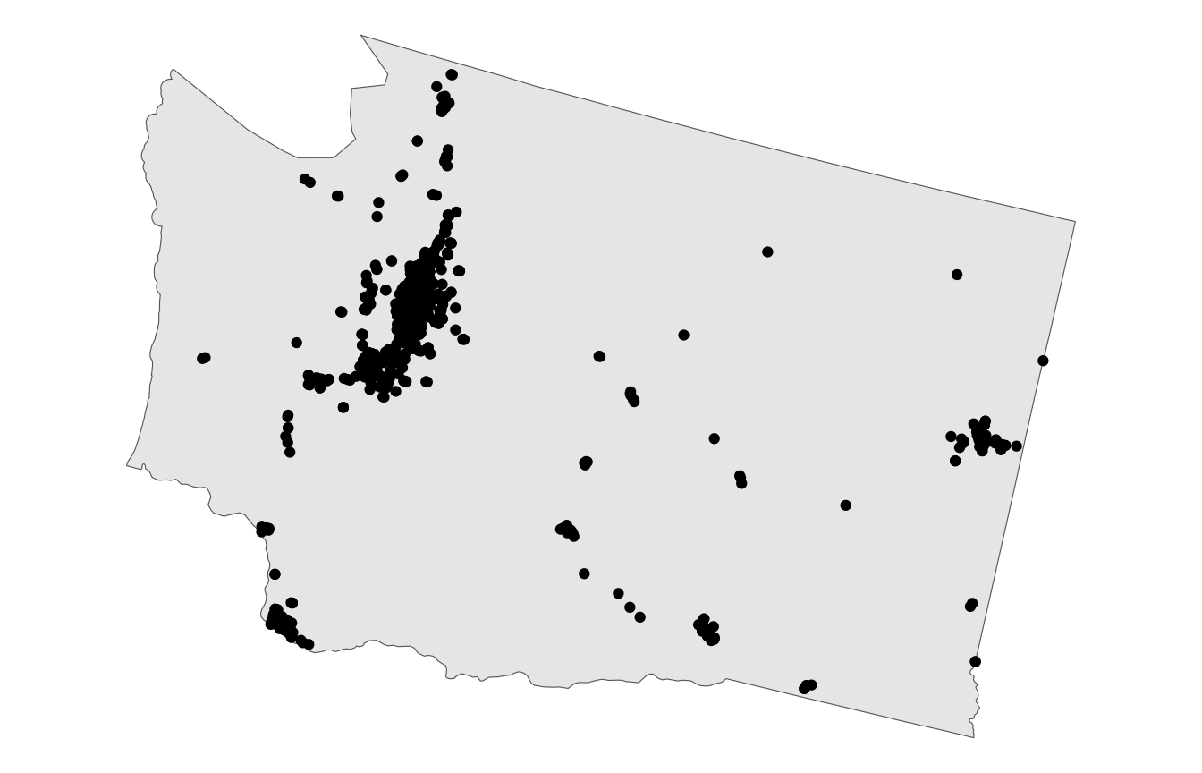
Spatial Joining
- Joining two non-spatial datasets relies on a shared key that uniquely identifies each record in a table
Spatially joining data relies on shared geographic relations rather then a shared key
Like filter, these relations can be defined by a predicate
As with tabular data, mutating joins add data to the target object (x) from a source object (y).
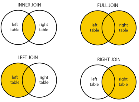
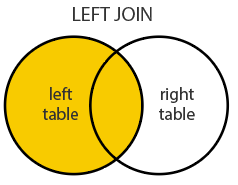
st_join
In
sfst_joinprovides this joining capacityBy default,
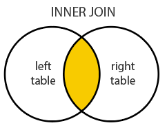
st_joinperforms a left join (Returns all records from x, and the matched records from y)It can also do inner joins by setting
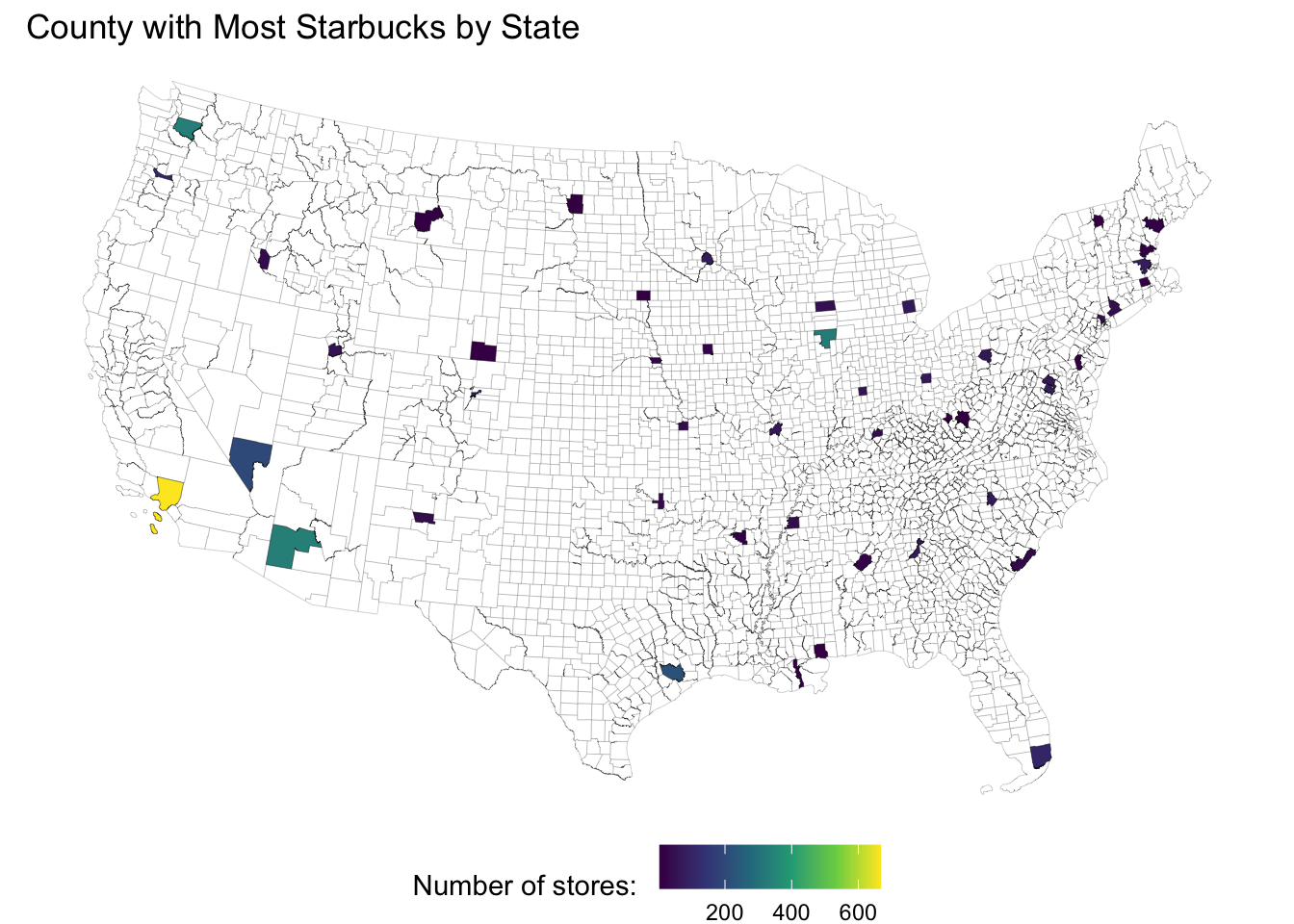
left = FALSE.Important: Many-to-many relationships create duplicate rows. In the Starbucks-counties example, a single Starbucks points at a county boundary may match multiple counties, creating multiple rows for that Starbucks.
The default predicate for
st_join(andst_filter) isst_intersects, but this can be changed with the.predicateargument to use other spatial relations likest_touches,st_within, etc.
The default predicate for
st_join(andst_filter) isst_intersectsThis can be changed with the join argument (see
?st_joinfor details).
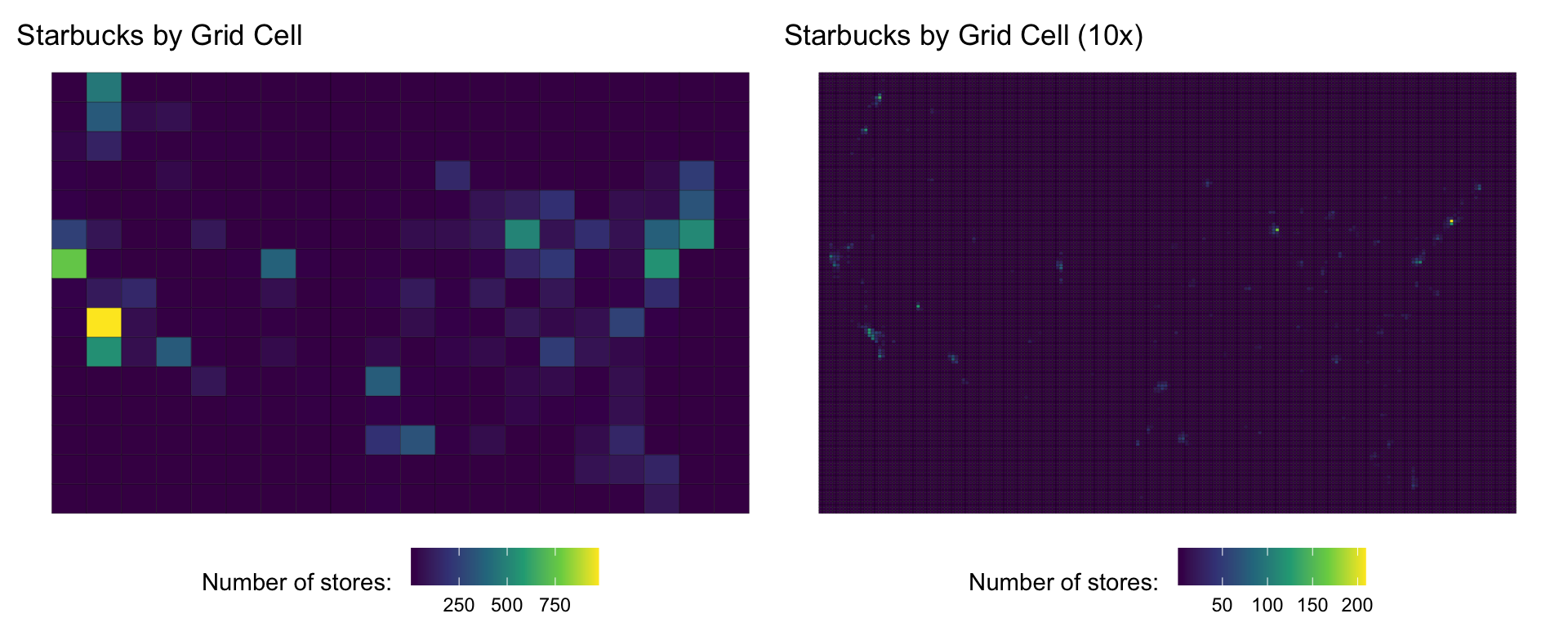
Tessellation and Aggregation (Sneek Peak)
- The same Starbucks data can be aggregated into different tessellation schemes
- This demonstrates how the choice of geographic units affects analysis results:
Clipping
Clipping is a form of subsetting that involves changing the geometry of at least some features.
Clipping can only apply to features more complex than points: (lines, polygons and their ‘multi’ equivalents).
Spatial Subsetting
- By default the data.frame subsetting methods we’ve seen (e.g
[,]) implementsst_intersection
Buffering
- A buffer is a zone of a specified distance around a geometry
st_buffer()expands or contracts geometries by a given distance- Useful for proximity analysis and creating zones of influence
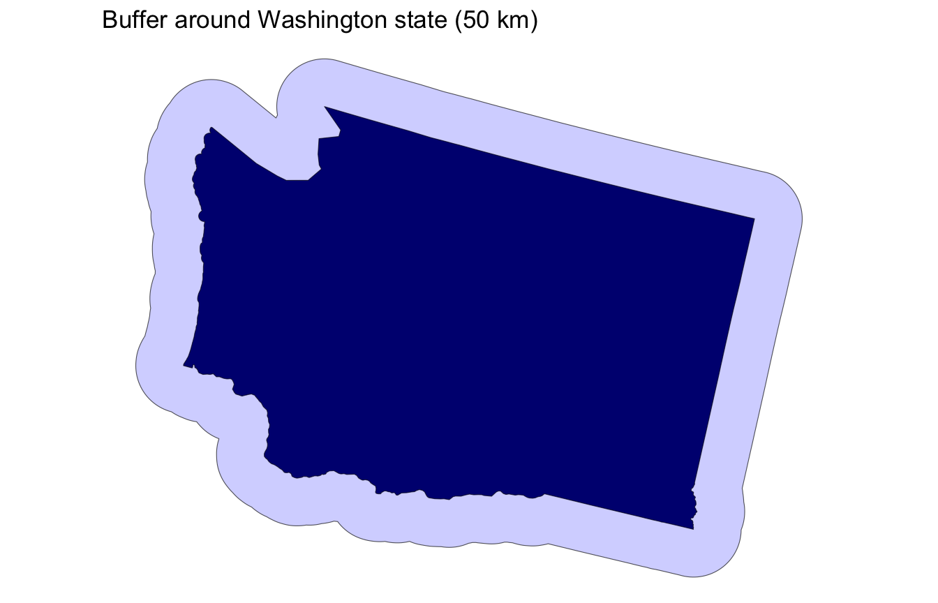
- Buffers are often combined with predicates for analysis like “find all cities within 100 km of a river”
Ramer–Douglas–Peucker
Mark the
firstandlastpoints as keptFind the point,
pthat is the farthest from the first-last line segment. If there are no points between first and last we are done (the base case)If
pis closer thantoleranceunits to the line segment then everything between first and last can be discardedOtherwise, mark p as kept and repeat steps 1-4 using the points between first and p and between p and last (the call to recursion)

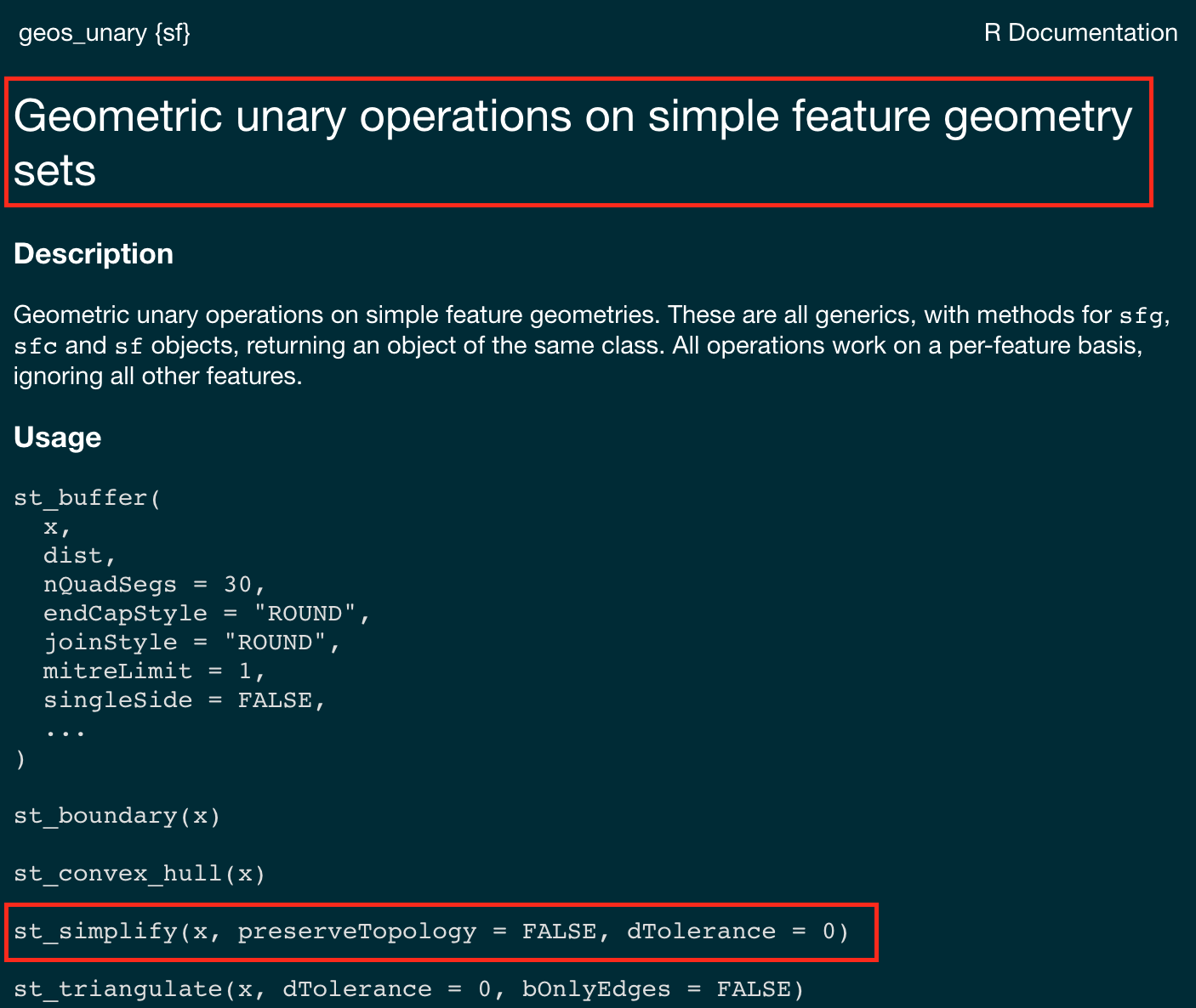
st_simplify
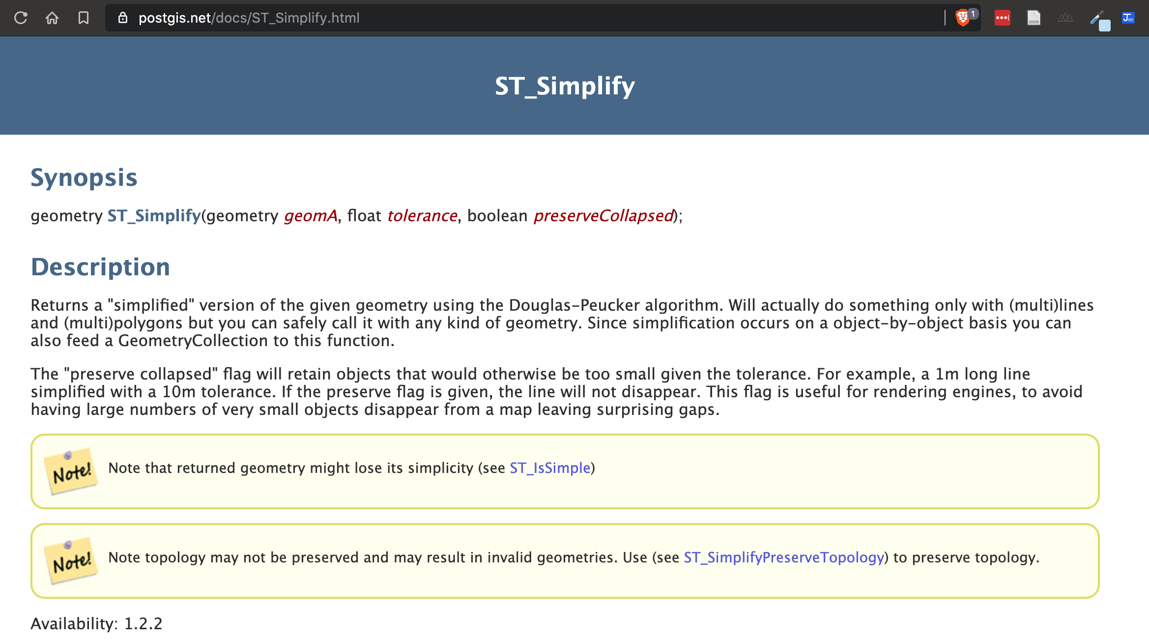
st_simplify
sfprovidesst_simplify, which uses the GEOS implementation of the Douglas-Peucker algorithm to reduce the vertex count.st_simplifyuses thedToleranceto control the level of generalization in map units (see Douglas and Peucker 1973 for details).Note on CRS: We use EPSG:5070 (USA Contiguous Albers Equal Area projection) for these examples because it preserves area and provides consistent distance measurements across the continental US, making tolerance values meaningful and comparable.
Performance Impact of Simplification
- Simplification dramatically reduces computational complexity for subsequent operations
#> Original points: 11292
#> After 10 km tolerance: 220
#> After 100 km tolerance: 27
#> After 1000 km tolerance: 4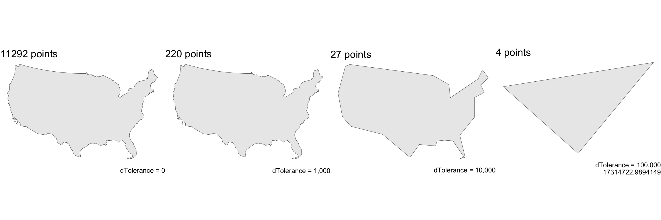
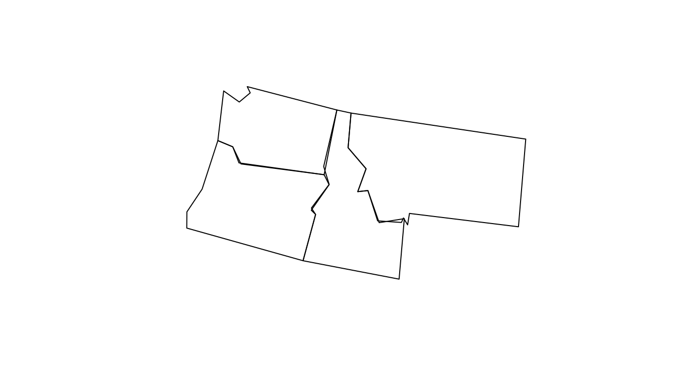
A limitation with Douglas-Peucker (therefore st_simplify) is that it simplifies objects on a per-geometry basis.
This means the ‘topology’ is lost, resulting in overlapping and disconnected geometries.
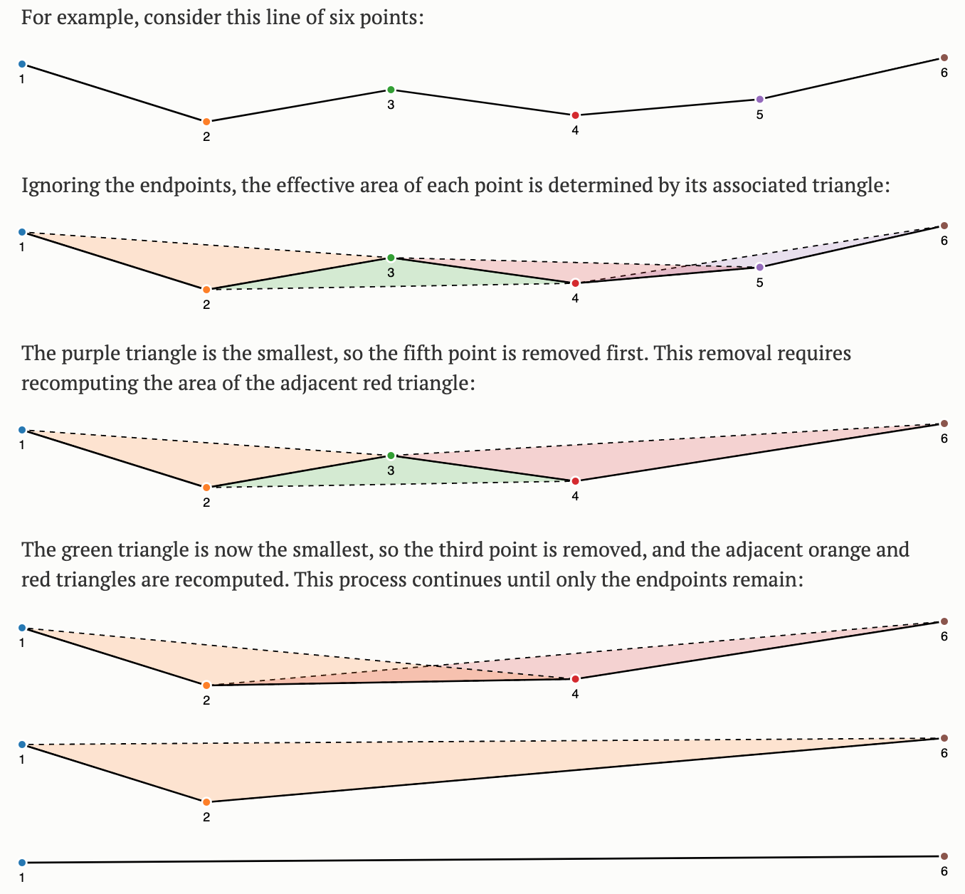
Visvalingam
- The Visvalingam algorithm overcomes some limitations of the Douglas-Peucker algorithm (Visvalingam and Whyatt 1993).
- it progressively removes points with the least-perceptible change.
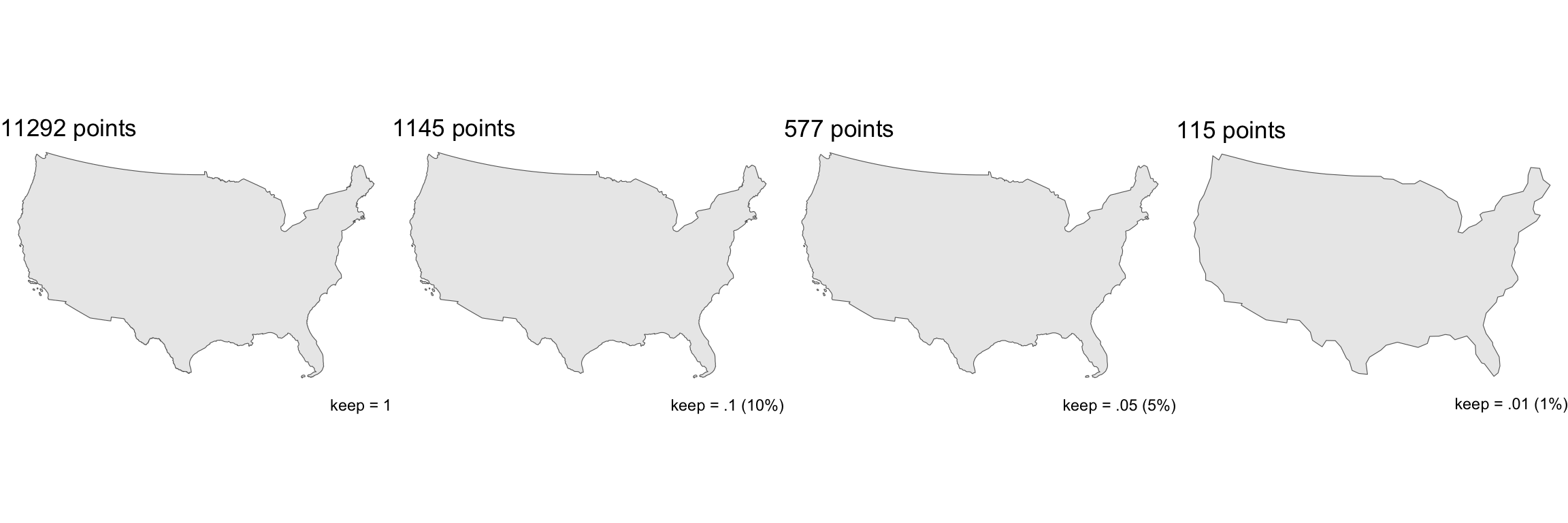
- Simplification often allows the elimination of 95% or more points while retaining sufficient detail for visualization and often analysis
rmapshaper
In R, the rmapshaper package implements the Visvalingam algorithm in the ms_simplify function.
- The
ms_simplifyfunction is a wrapper around themapshaperJavaScript library (created by lead viz experts at the NYT)
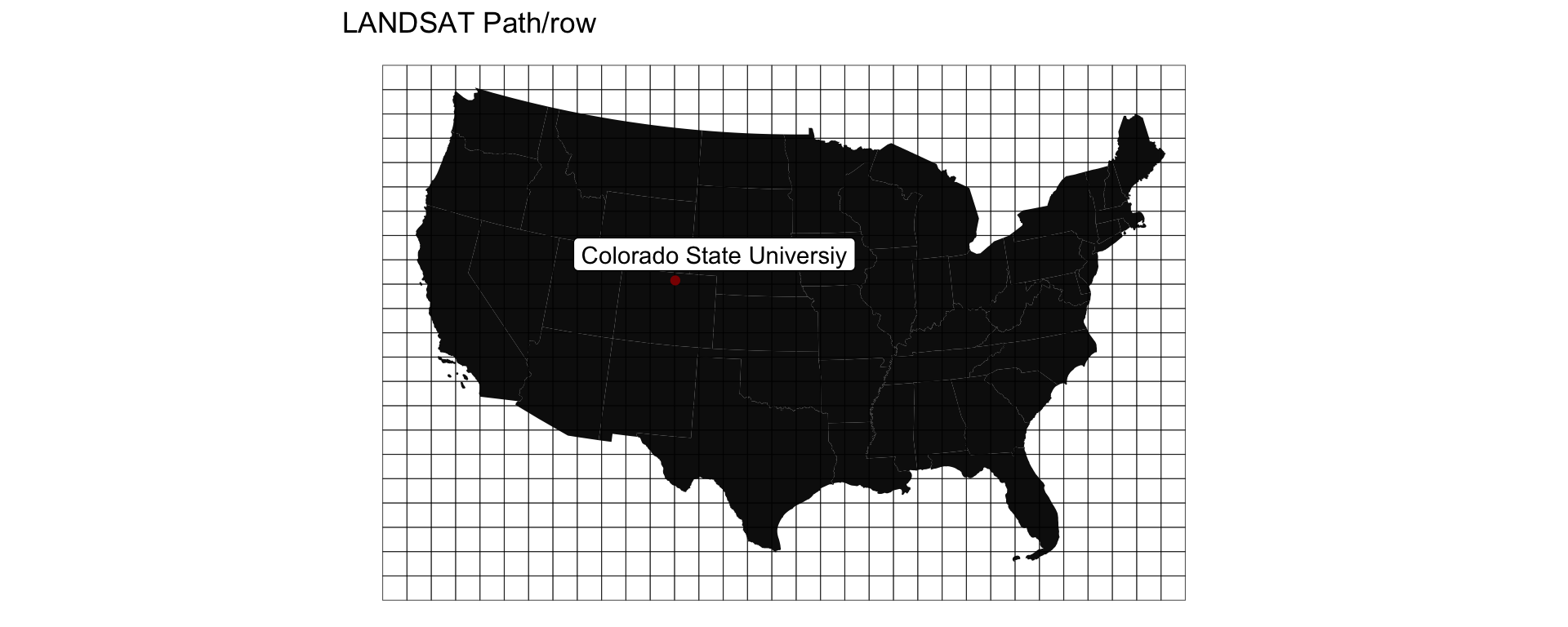
LANDSAT Path Row
- Serves tiles based on a path/row index
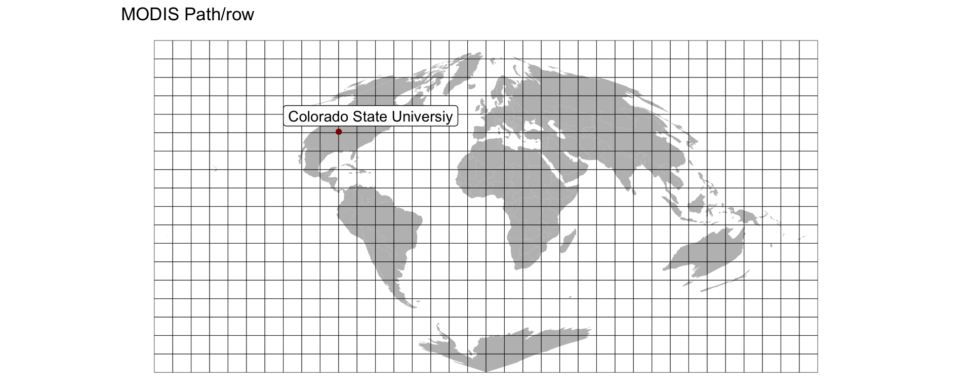
MODIS Sinisoial Grid
- Serves tiles based on a path/row index
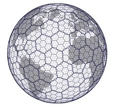
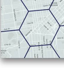
Uber Hex Addressing
- Breaks the world into Hexagons…
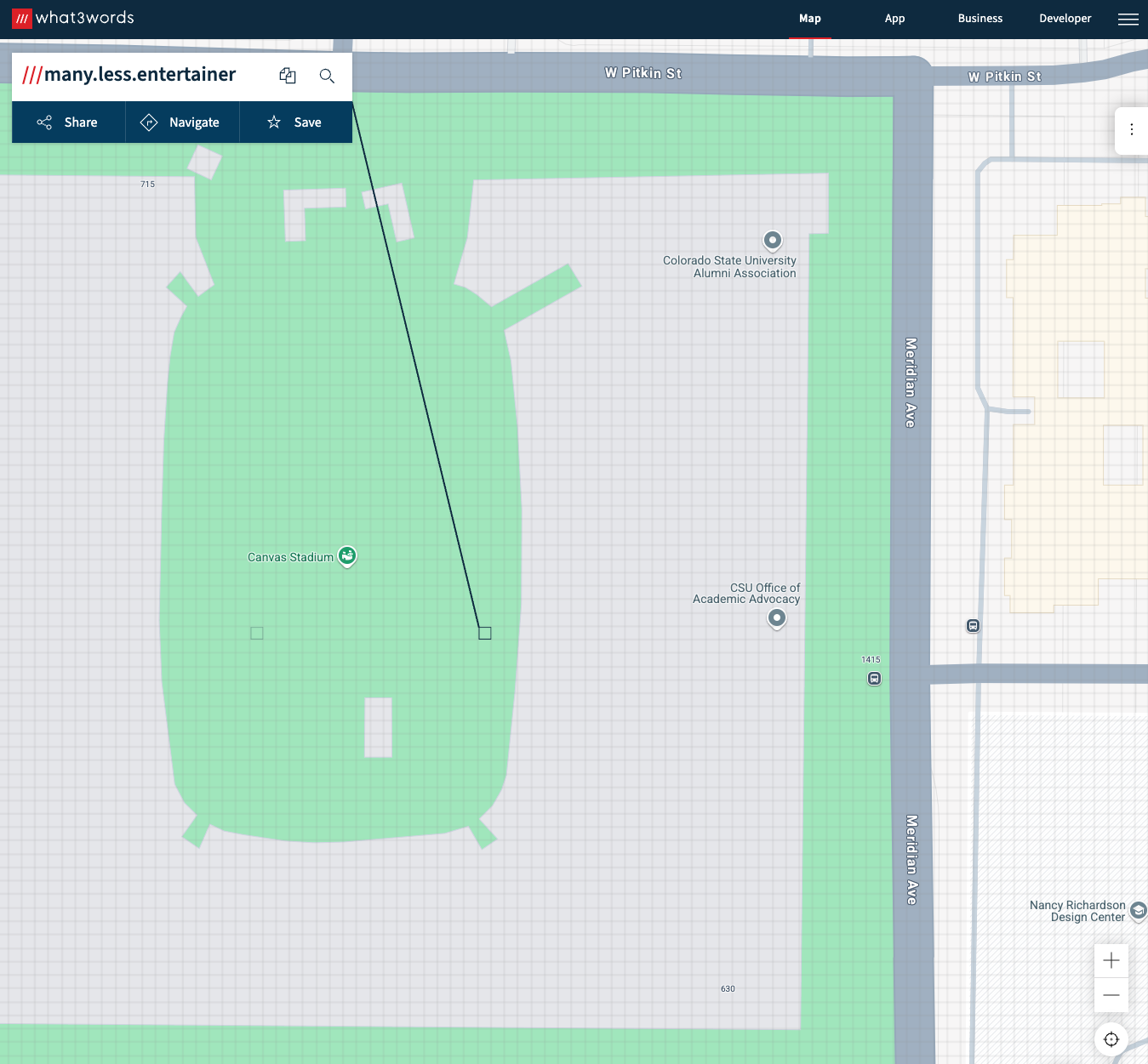
what3word
- Breaks the world into 3m grids encoded with unique 3 word strings
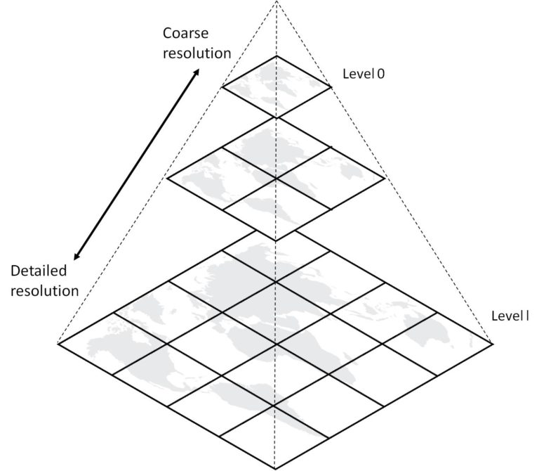
Map Tiles / slippy maps / Pyramids
- Use XYZ where Z is a zoom level …
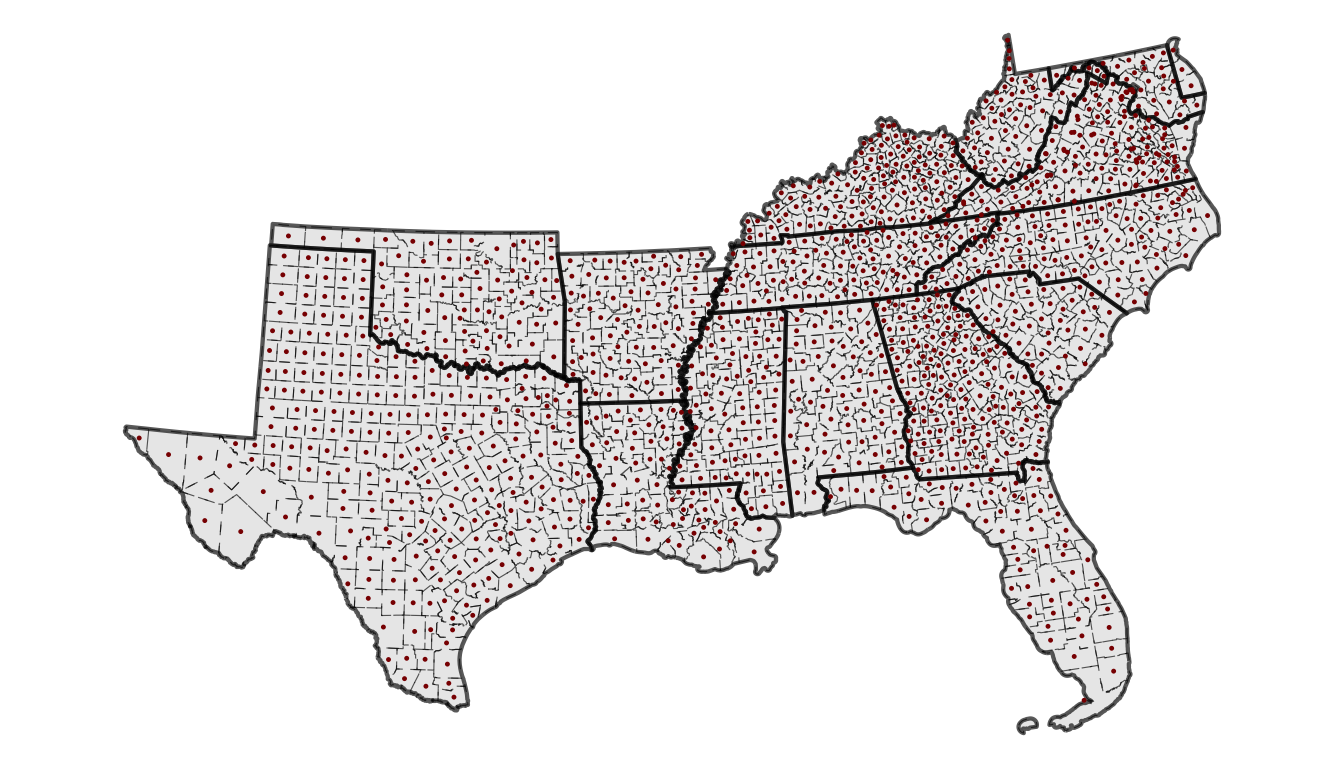
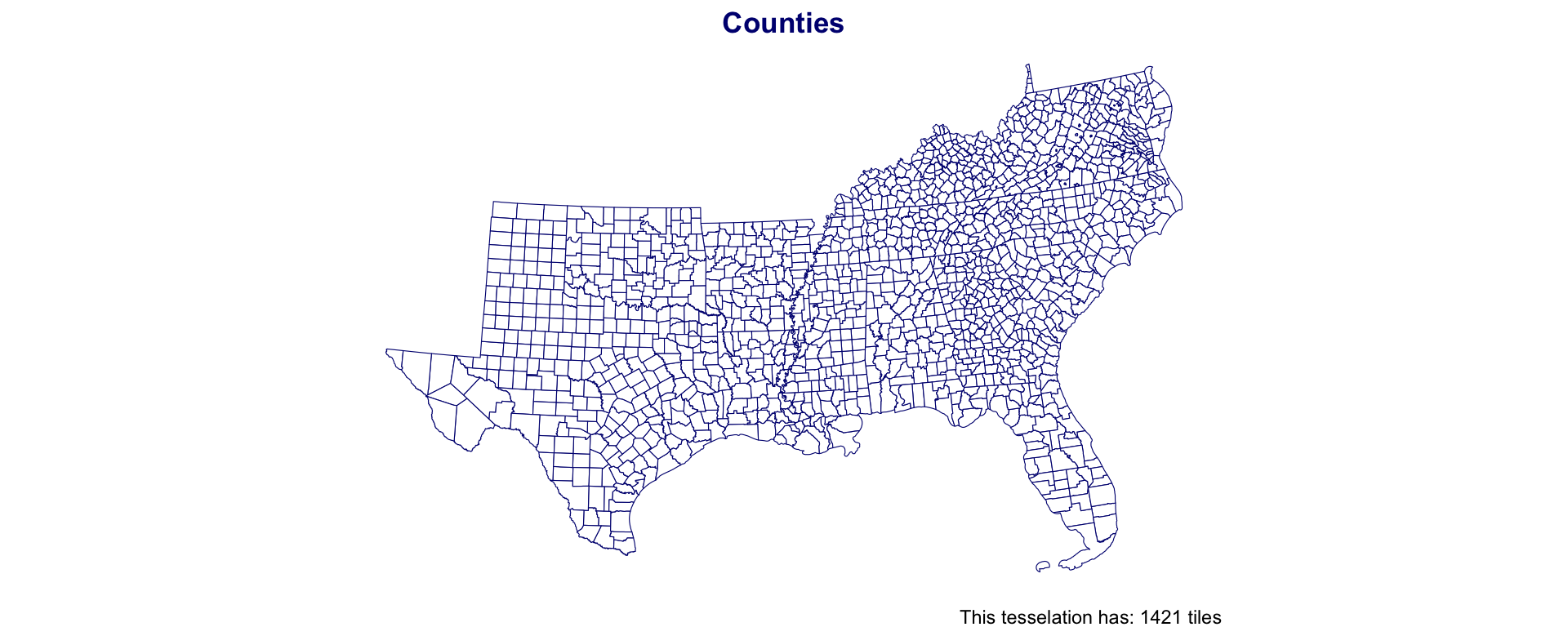
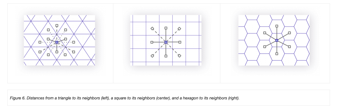
Our Data for today …
Southern Counties
Unioned to States using dplyr
South County Centroids
Southern Coverage: County
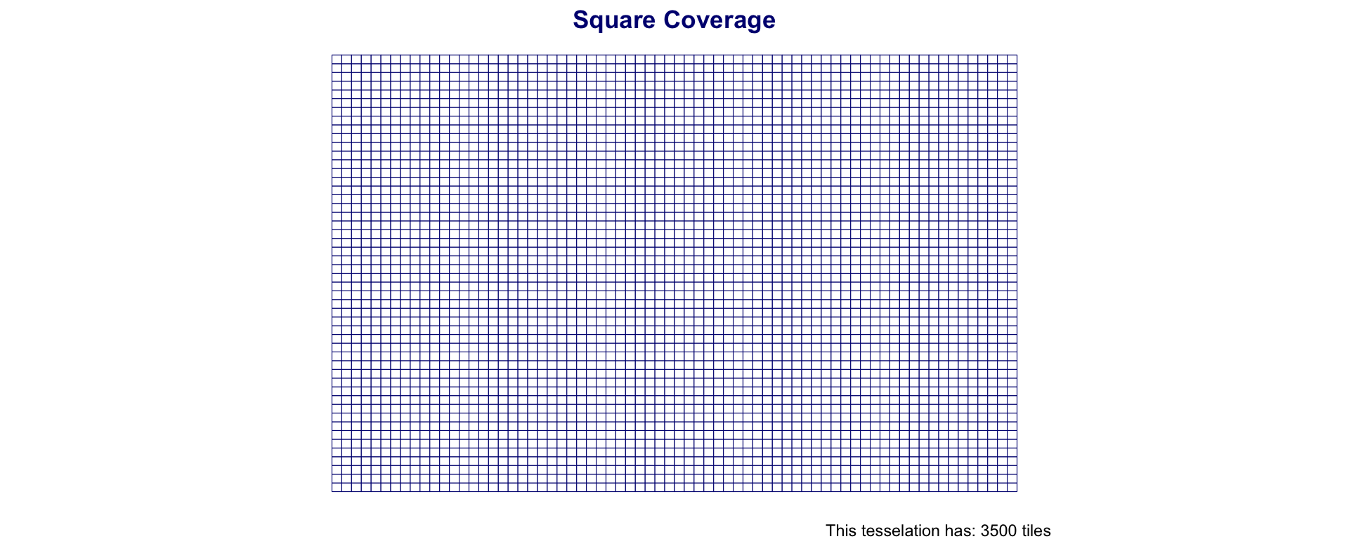
Southern Coverage: Square
Southern Coverage: Hexagon

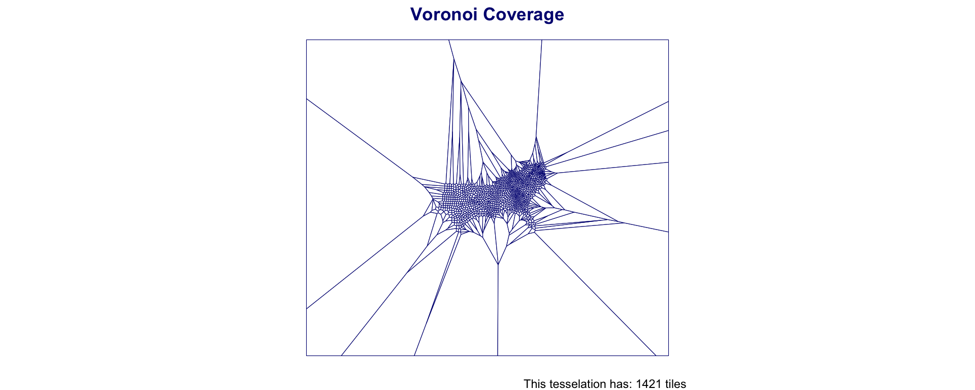
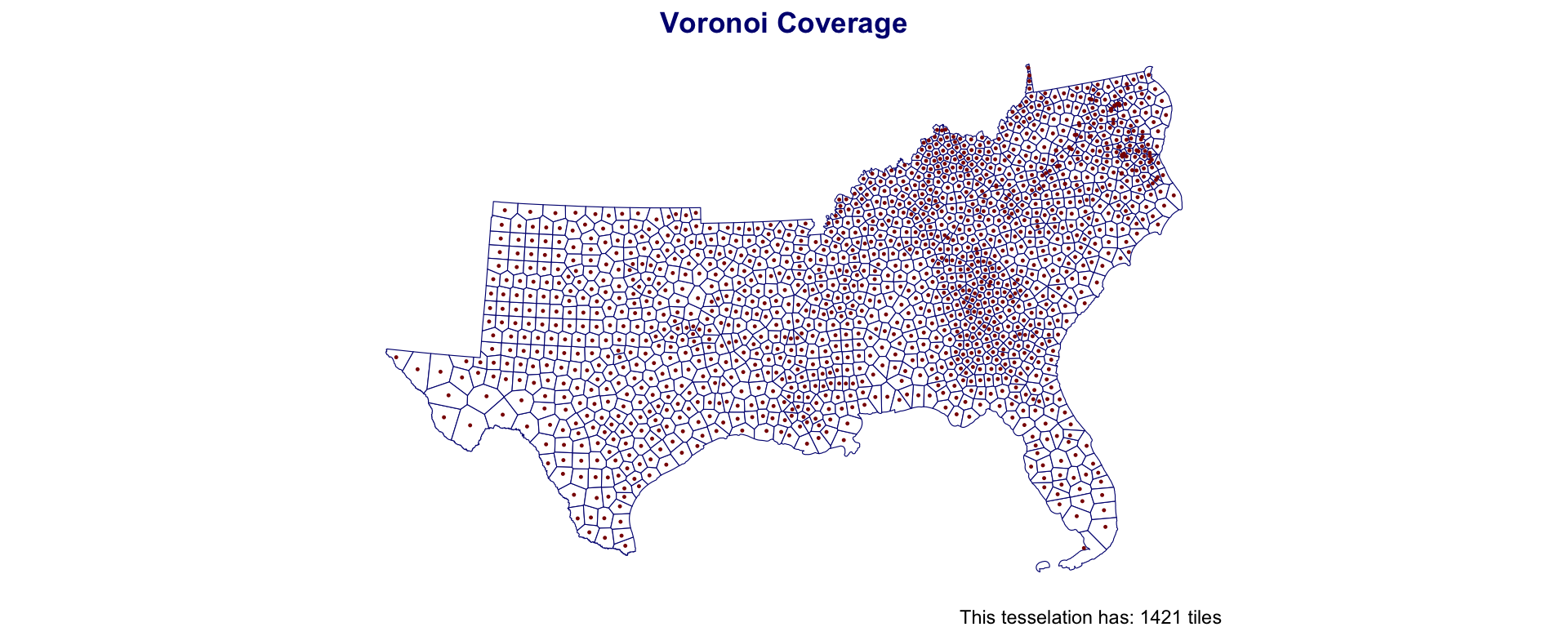
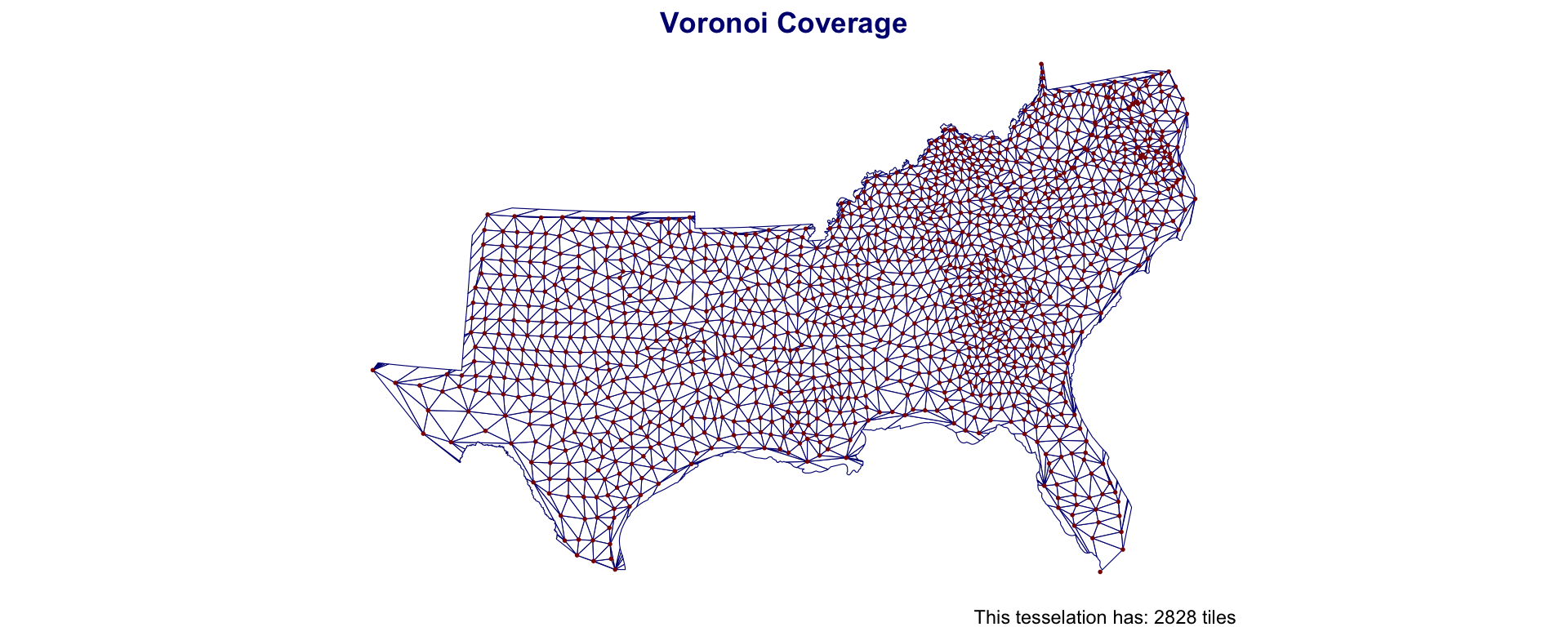
Voronoi Polygons
Voronoi/Thiessen polygon boundaries define the area closest to each anchor point relative to all others
They are defined by the perpendicular bisectors of the lines between all points.
Voronoi Polygons
Voronoi Polygons
- Usefull for tasks such as:
- nearest neighbor search,
- facility location (optimization),
- largest empty areas,
- path planning…
- Also useful for simple interpolation of values such as rain gauges,
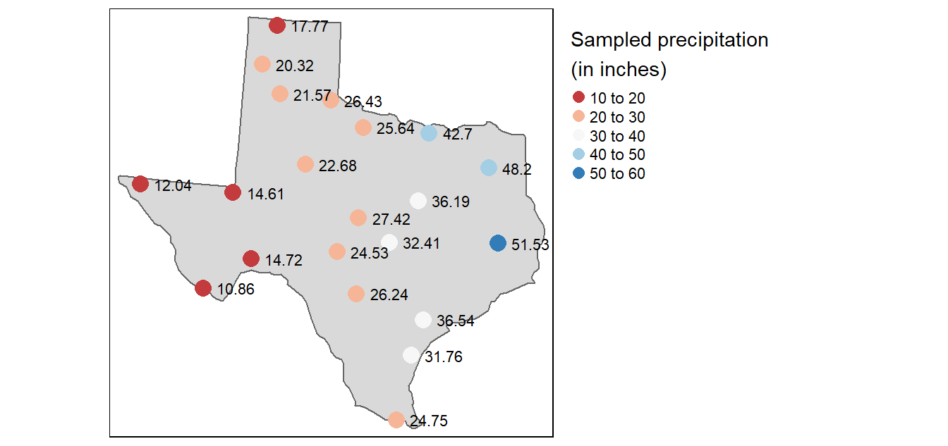
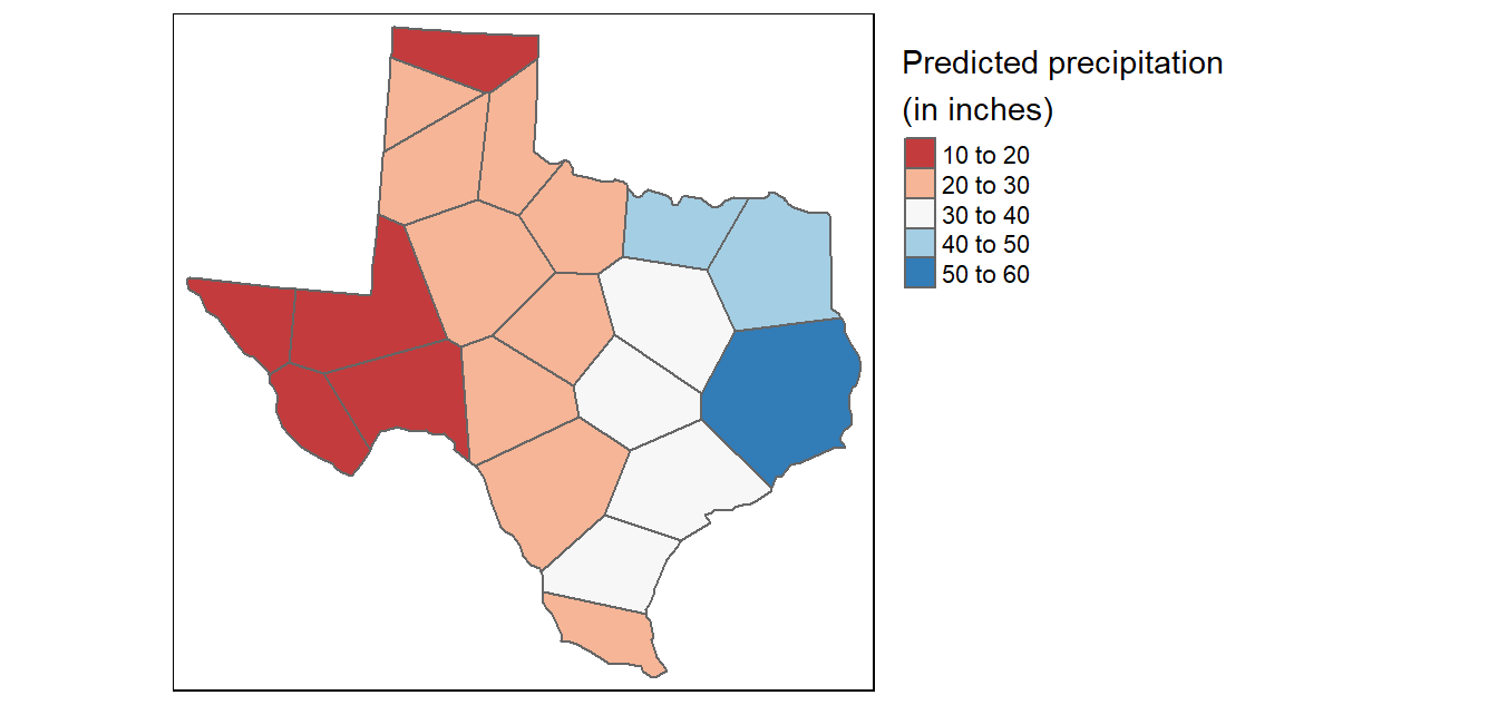
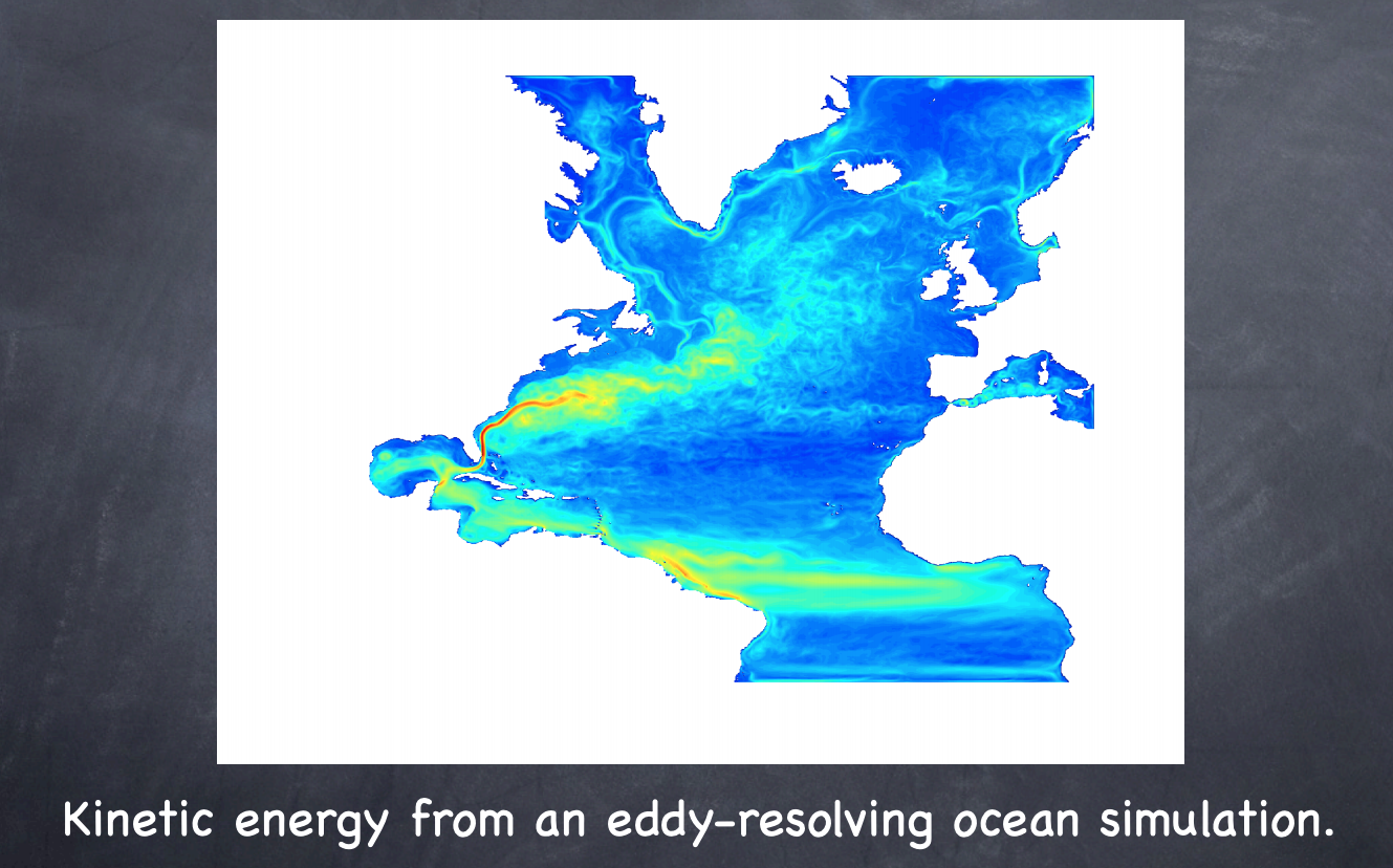
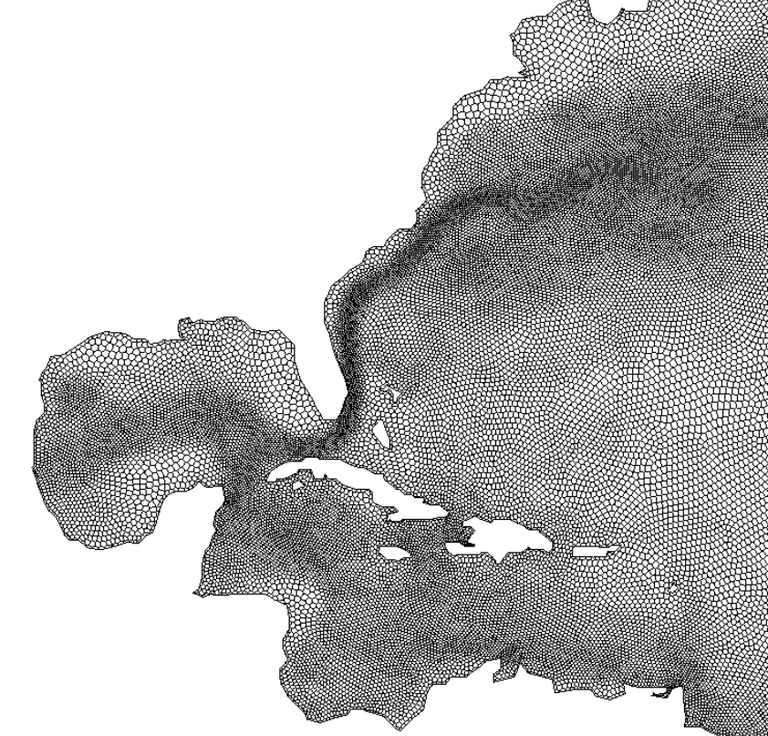
Often used in numerical models and simulations
Southern Coverage: Voronoi
Southern Coverage: Voronoi
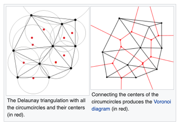
Delaunay triangulation
- A Delaunay triangulation for a given set of points (P) in a plane, is a triangulation DT(P), where no point is inside the circumcircle of any triangle in DT(P).
Delaunay triangulation
The Delaunay triangulation of a discrete POINT set corresponds to the dual graph of the Voronoi diagram.
The circumcenters (center of circles) of Delaunay triangles are the vertices of the Voronoi diagram.
Used in landscape evaluation and terrian modeling
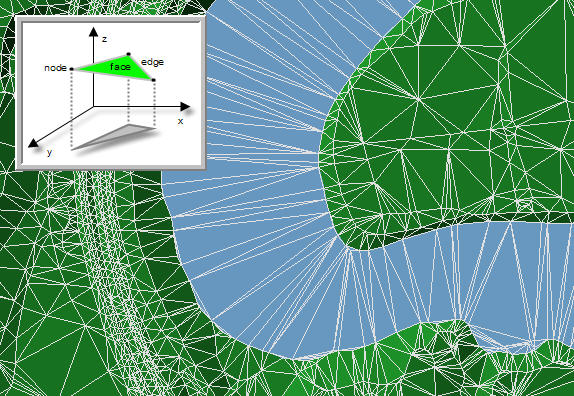
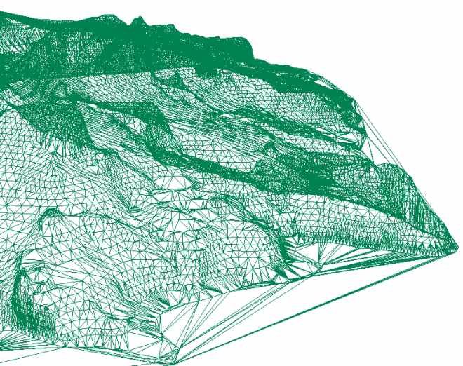
Southern Coverage: Triangles
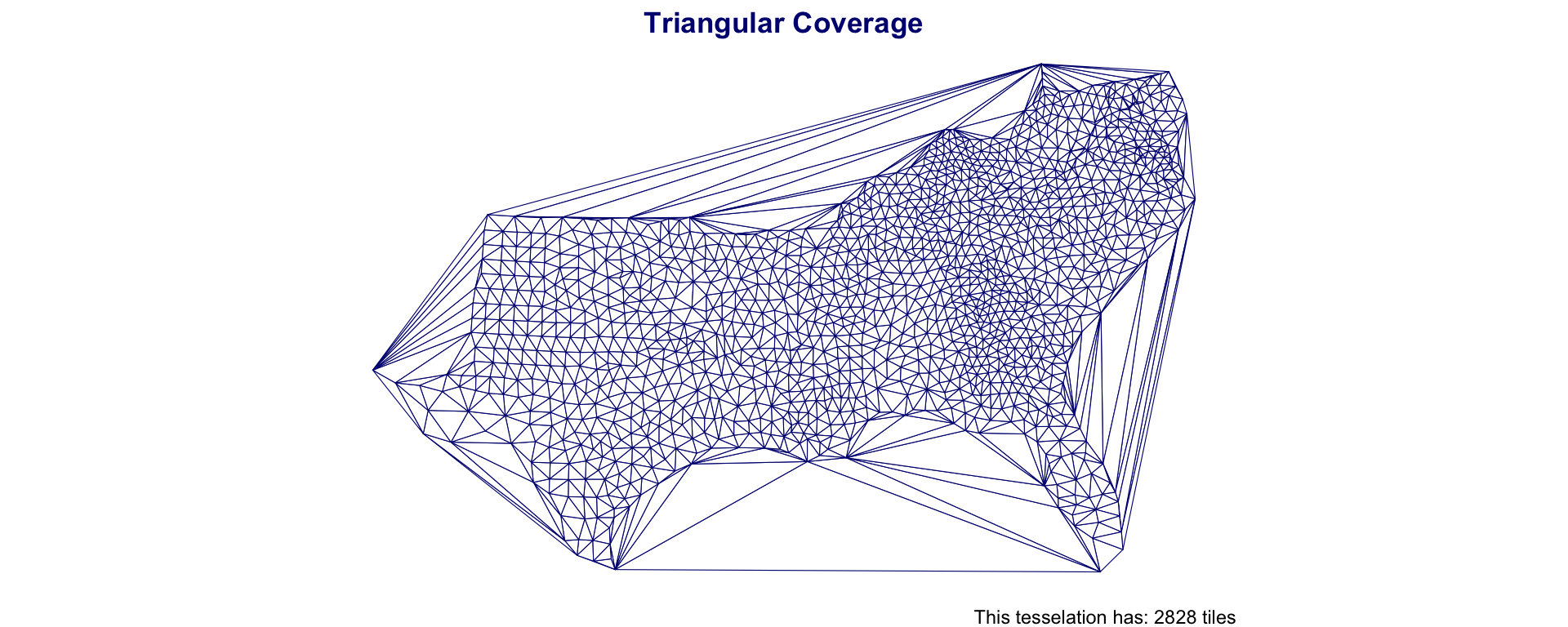
Southern Coverage: Triangles
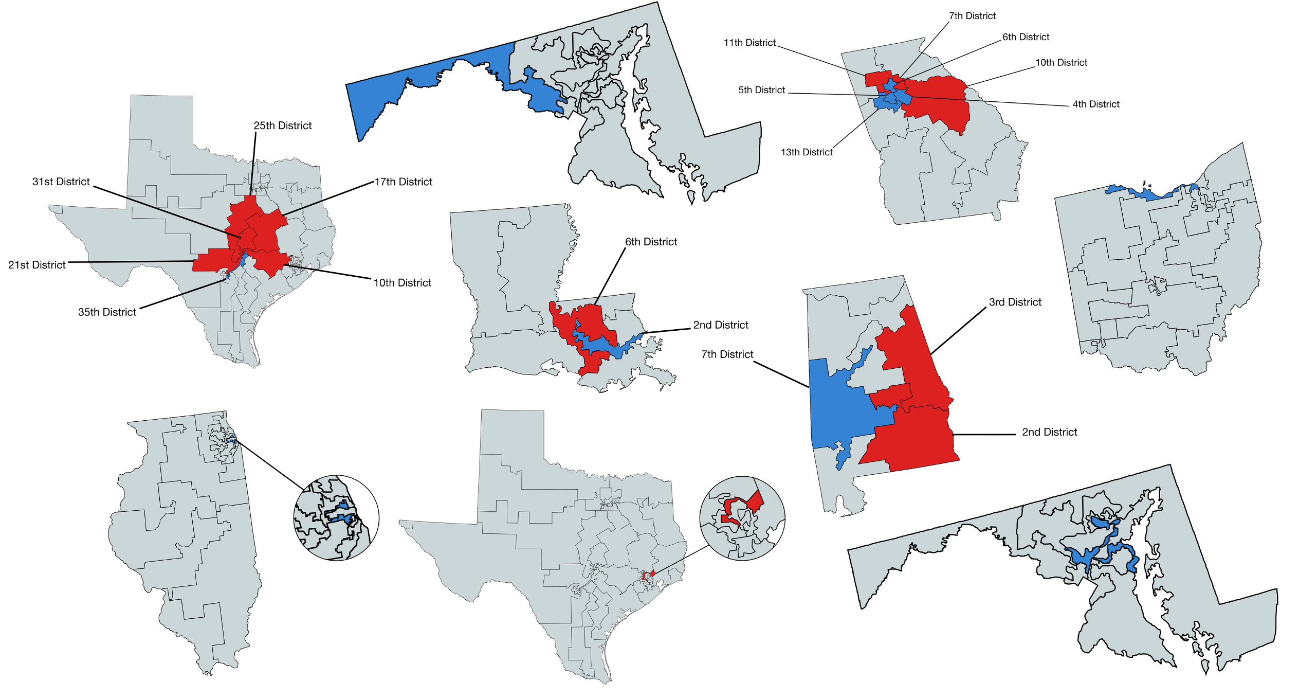
Modifiable areal unit problem (MAUP)
The modifiable areal unit problem (MAUP) is a source of statistical bias that can significantly impact the results of statistical hypothesis tests.
MAUP affects results when point-based measures are aggregated into districts.
The resulting summary values (e.g., totals or proportions) are influenced by both the shape and scale of the aggregation unit.
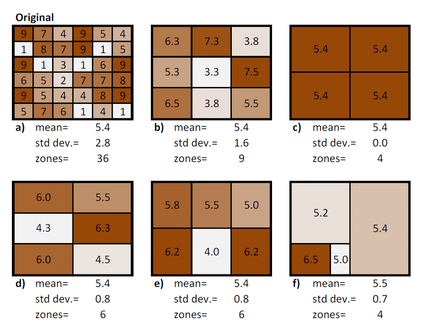
Examples
Moran’s I example: map + takeaway
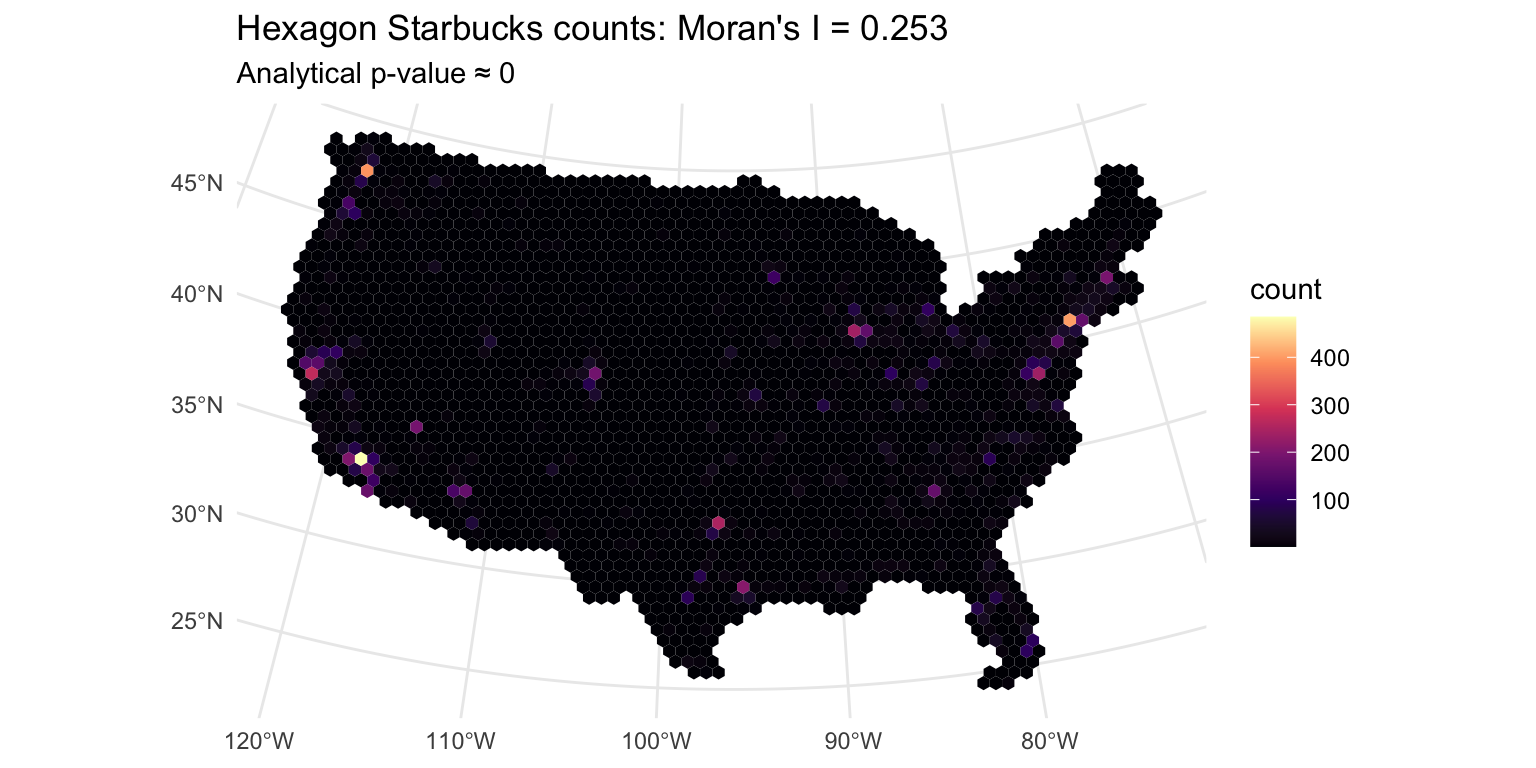
Teaching takeaway: similar values are clustering in space, so this pattern is not well described as iid randomness.
Interpretation in plain English: places with lots of Starbucks tend to be near places with lots of Starbucks; places with few tend to be near places with few.
So what for water resources research?
- if flood losses cluster, response planning should be regional, not purely local
- if model residuals cluster, validation should account for spatial dependence
- if hydrologic signatures cluster, regionalization may be defensible — but only at the right scale
Spatial lag: what your neighbors look like
The spatial lag is the weighted neighborhood average:
\[ ext{lag}(x) = W x\]
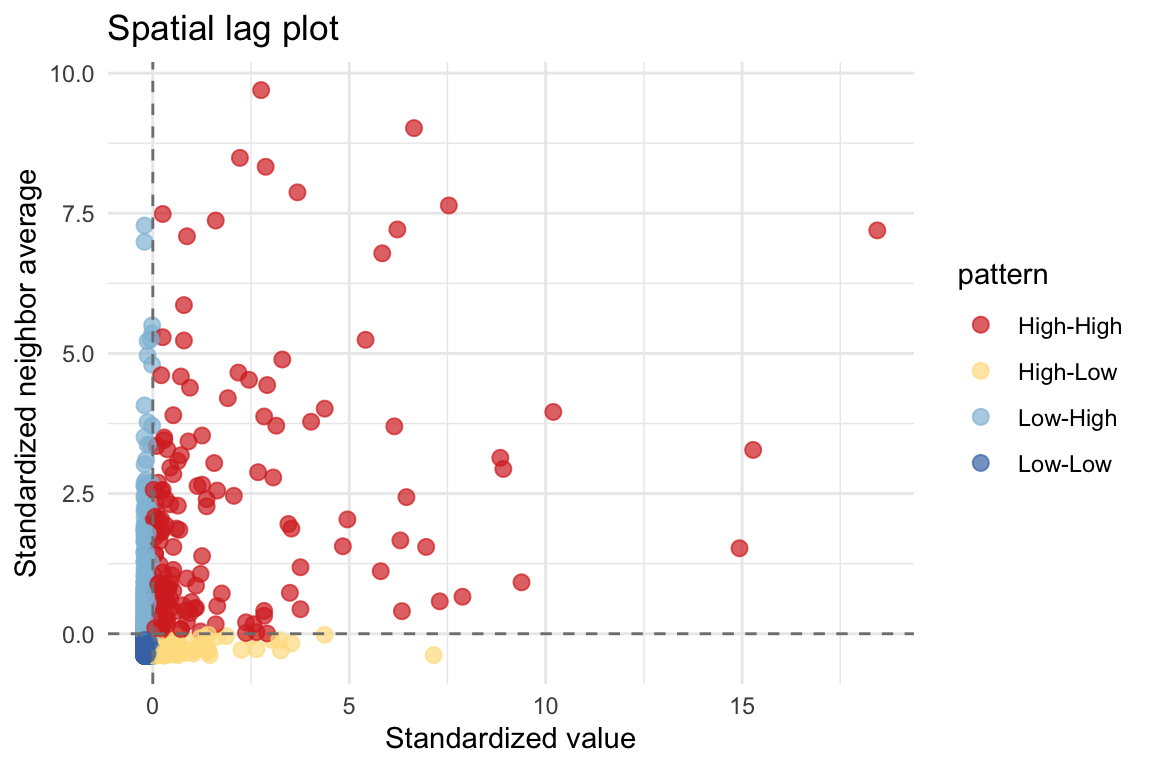
This gives local intuition:
- upper-right = high values near high values
- lower-left = low values near low values
- off-diagonal = local mismatch or transition
Local clustering intuition
A global Moran’s I gives one number for the whole map.
A local view asks:
Where are the high-high and low-low areas?
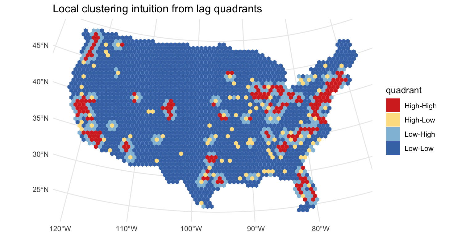
This is a useful bridge to LISA without overloading the first lesson with full local significance testing.
So what? Local patterns are often what matter operationally: where should we investigate, intervene, monitor, or transfer information with caution?