(ny <- AOI::aoi_get(state = "NY") |>
   st_transform(5070) |>
   dplyr::select(name))
#> Simple feature collection with 1 feature and 1 field
#> Geometry type: MULTIPOLYGON
#> Dimension:     XY
#> Bounding box:  xmin: 1319503 ymin: 2149150 xmax: 1997508 ymax: 2658544
#> Projected CRS: NAD83 / Conus Albers
#>       name                       geometry
#> 1 New York MULTIPOLYGON (((1661336 263...Week 4
Raster Data
Result:
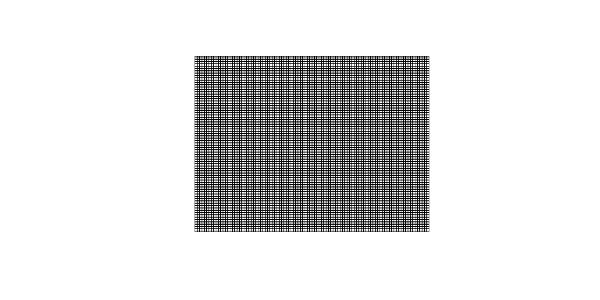
Extents can be discretized in a number of ways:
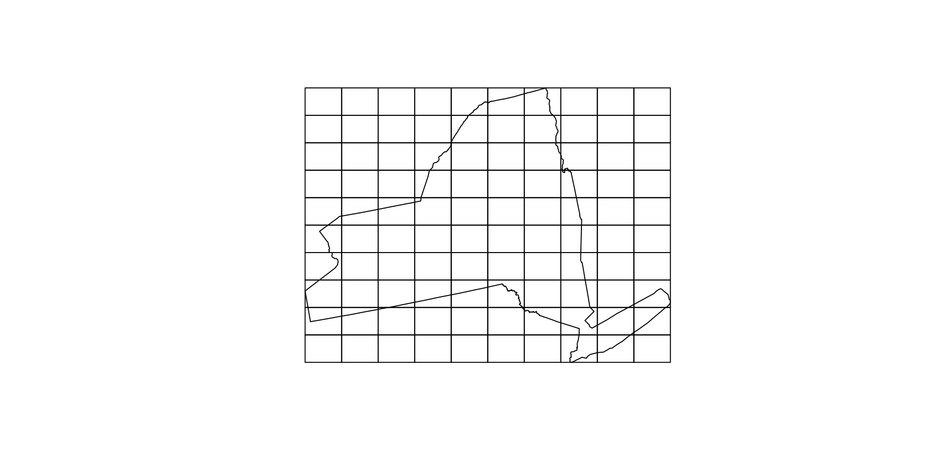
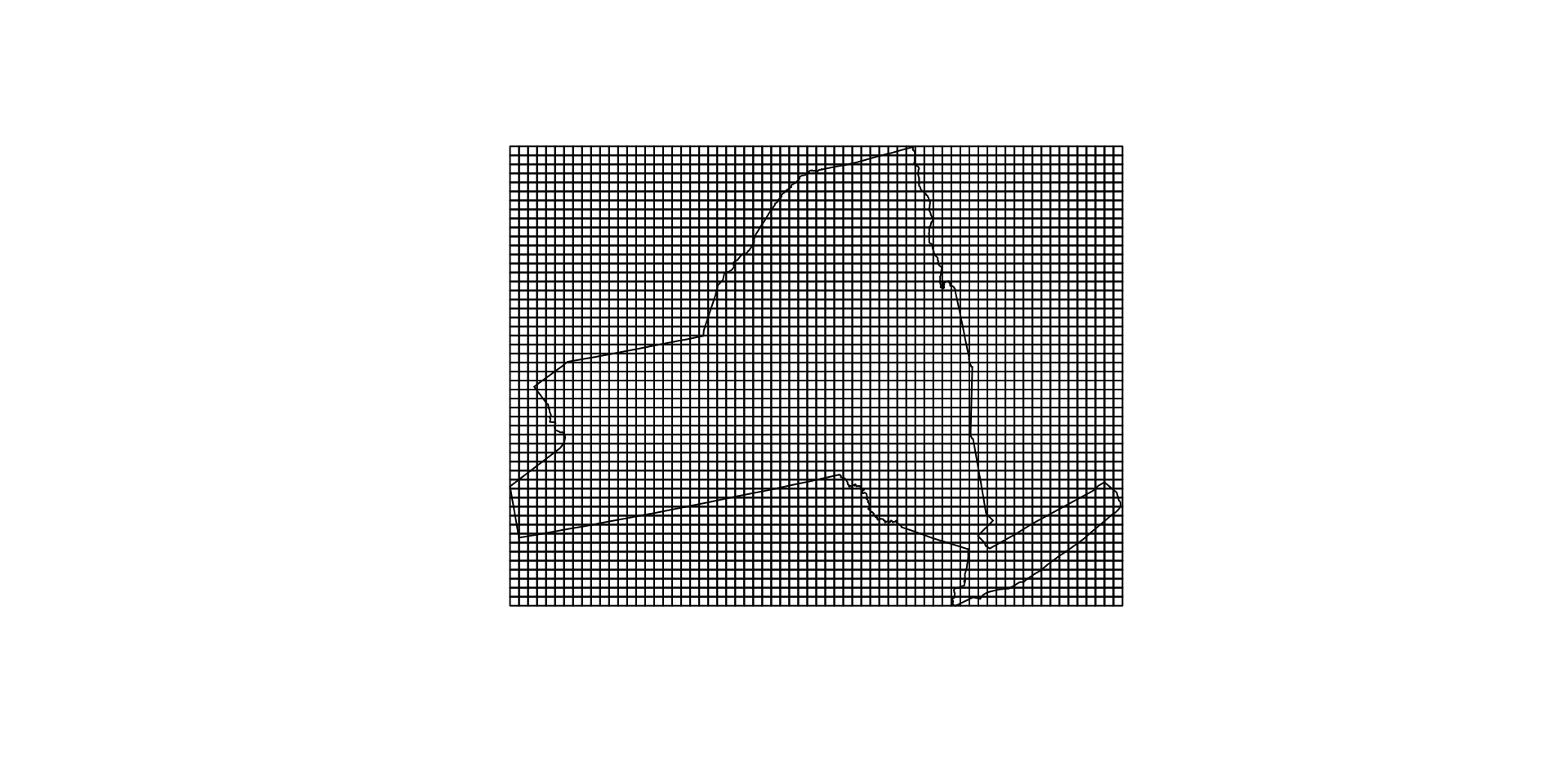
Alternative representation
Regular grids can also be indexed by their centroids
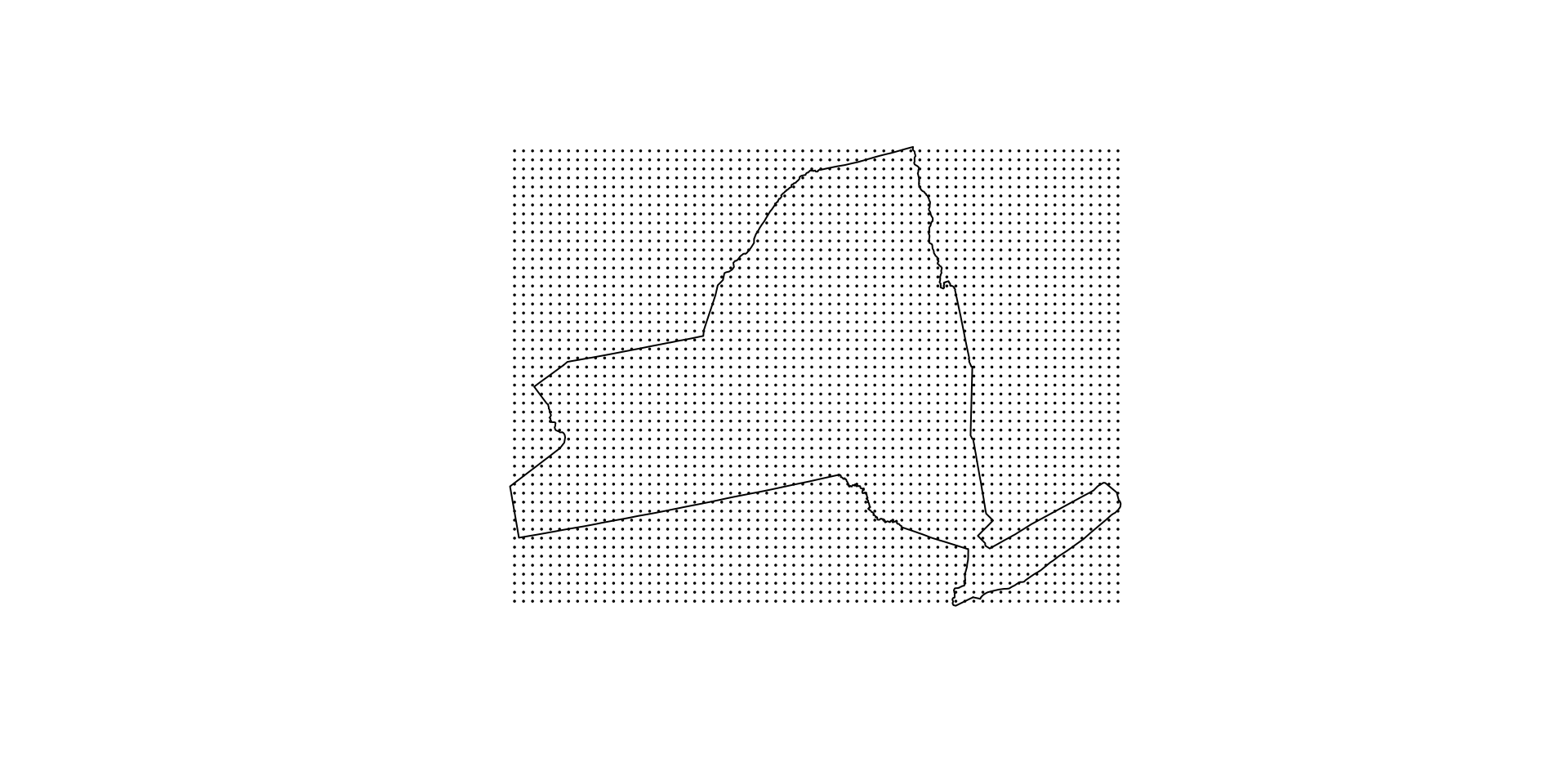
Equal area from centroid
We can use our voronoi diagram to show that the area closest to a cell centroid is the cell itself.

Many terms mean the same thing …
The entire raster is sometimes referred to as an “image”, “array”, “surface”, “matrix”, or “lattice” (Wise, 2000).
They all mean the same thing.
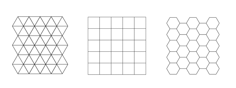
Cells of the raster are most often square, but may be rectangular (with differing resolutions in x and y directions) or other shapes that can be tessellated such as triangles and hexagons (Figure below from Peuquet, 1984).
Photos and Computers …
![]()
![]()
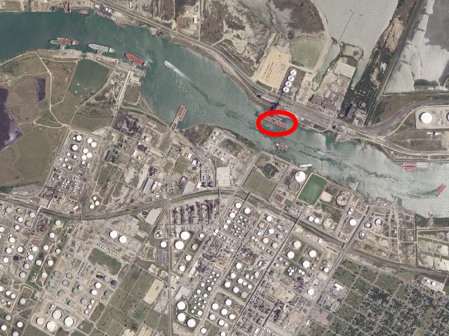
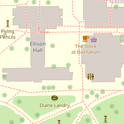
Aerial Imagery (really just a photo 😄)
What is stored in these cells?
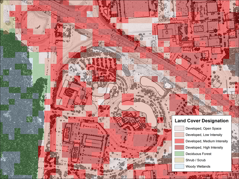
Categorical Values (integer/factor)
![]()
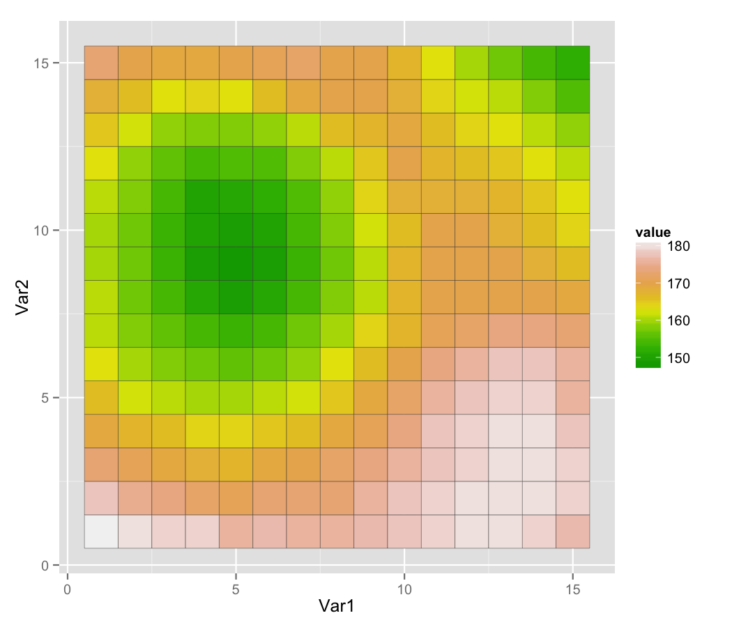
Continuous Values (numeric)
Spectral Values
- Either Color, or sensor
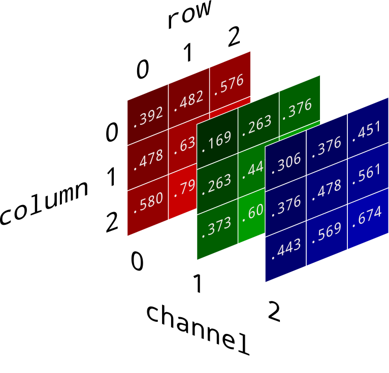
Pure RGB
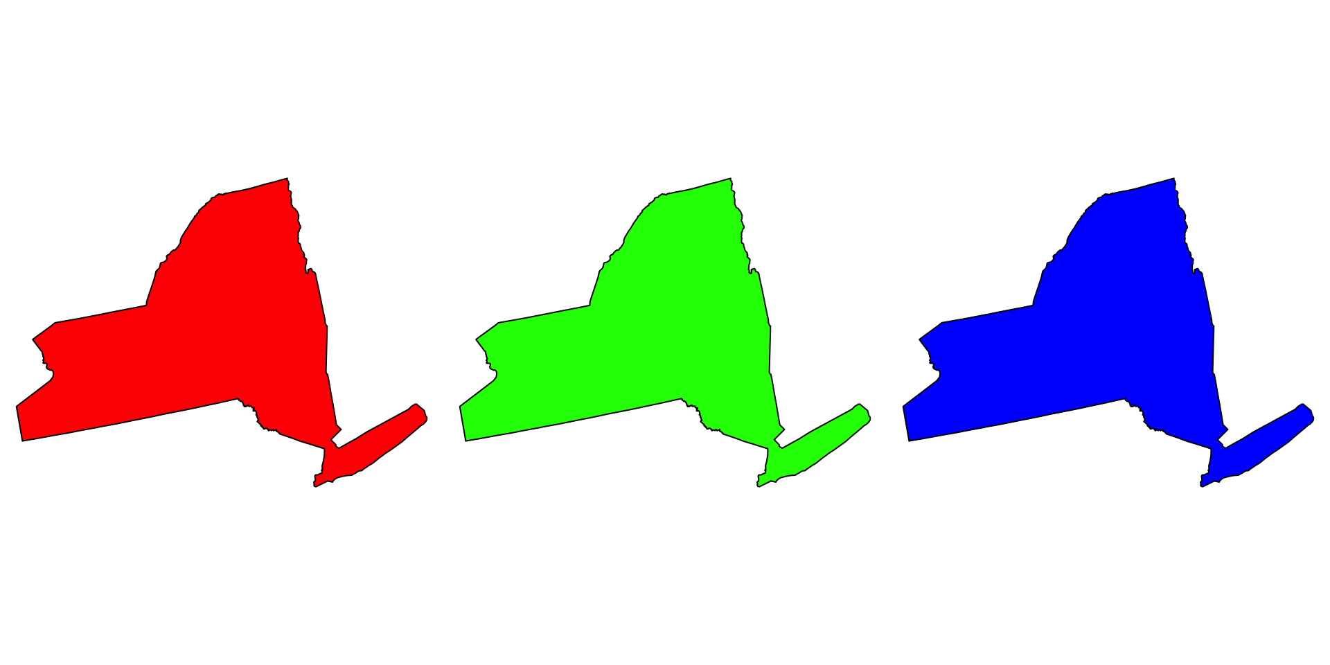
RGB values are what matter most for raster imagery in this course.
- Digital images store color with red, green, and blue channels.
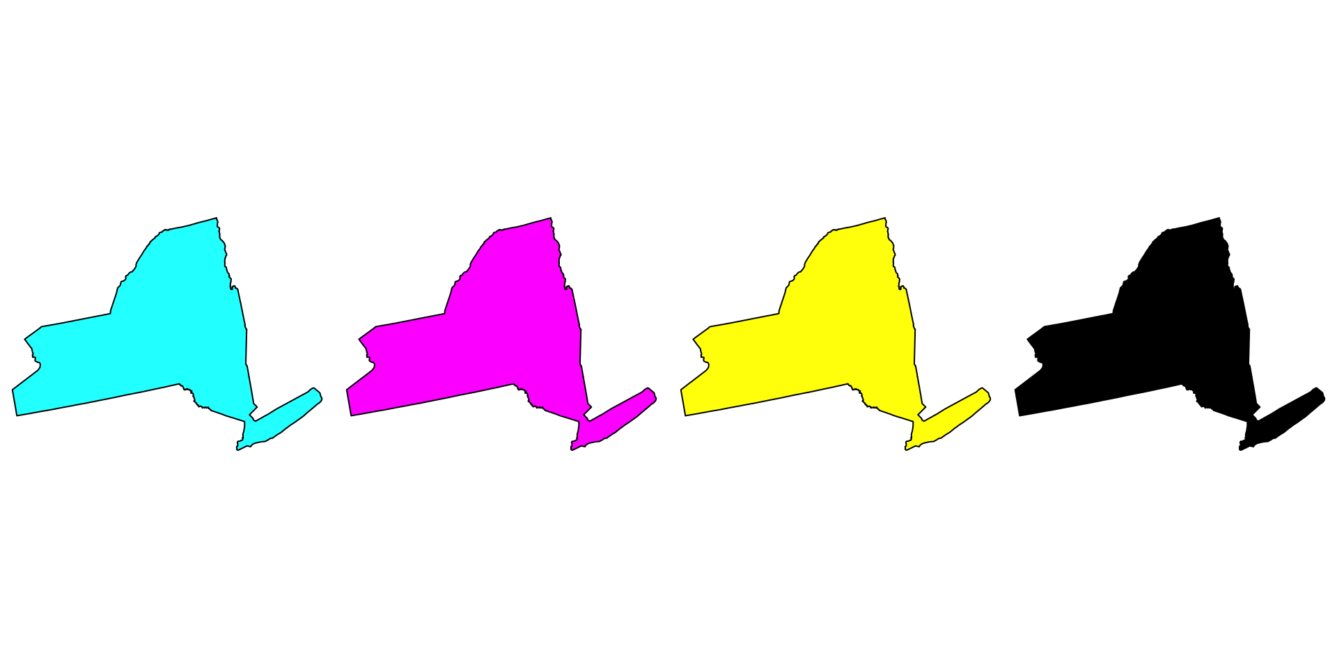
- Printers use a different system (CMYK), but the core idea is the same: color is encoded numerically.
- For us, the important takeaway is that image rasters store values by channel.
Why do we care?
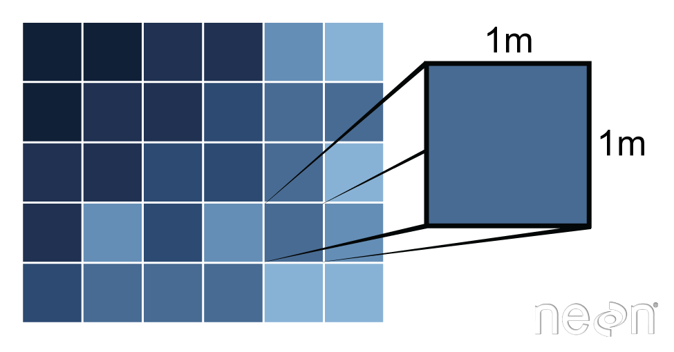
Pixels are the base unit of raster data and have a resolution
This is the X and the Y dimension of each cell in the units of the CRS
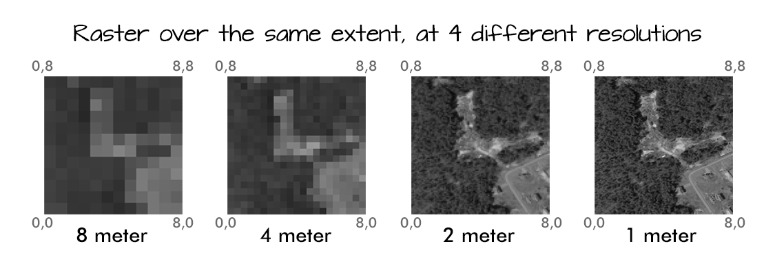
Resolution drives image clarity (granularity)
- Higher resolution (smaller cells) = more detail, but bigger data!
Raster images seek to discretize the real world into cell-based values
- Again either integer (categorical), continuous, or signal
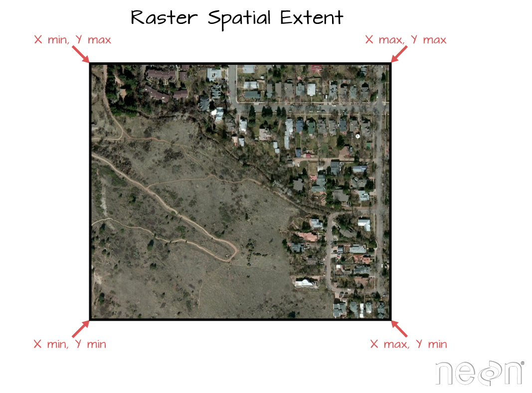
All rasters have an extent!
- This is the same extent as a bounding box
- Can be described as 4 values (xmin,ymin,xmax,ymax)
Implicit Coordinates
Unlike vector data, the raster data model stores cell coordinates indirectly.
Coordinates are derived from the raster origin, the resolution, and the cell index (for example, row 100 and column 150).
In practice, the column position determines movement in the x-direction and the row position determines movement in the y-direction. Cell-center coordinates are inferred from that structure rather than stored one by one.
So, any image (.png, .tif, .gif) can be read as a raster…
The raster is defined by the extent and resolution of the cells
To be spatial, the extent (and thus the coordinates) must be grounded in a CRS
(img = terra::rast('img/17-raster-extent.png'))
#> class       : SpatRaster
#> size        : 788, 1067, 4  (nrow, ncol, nlyr)
#> resolution  : 1, 1  (x, y)
#> extent      : 0, 1067, 0, 788  (xmin, xmax, ymin, ymax)
#> coord. ref. :
#> source      : 17-raster-extent.png
#> names       : 17-rast~xtent_1, 17-rast~xtent_2, 17-rast~xtent_3, 17-rast~xtent_4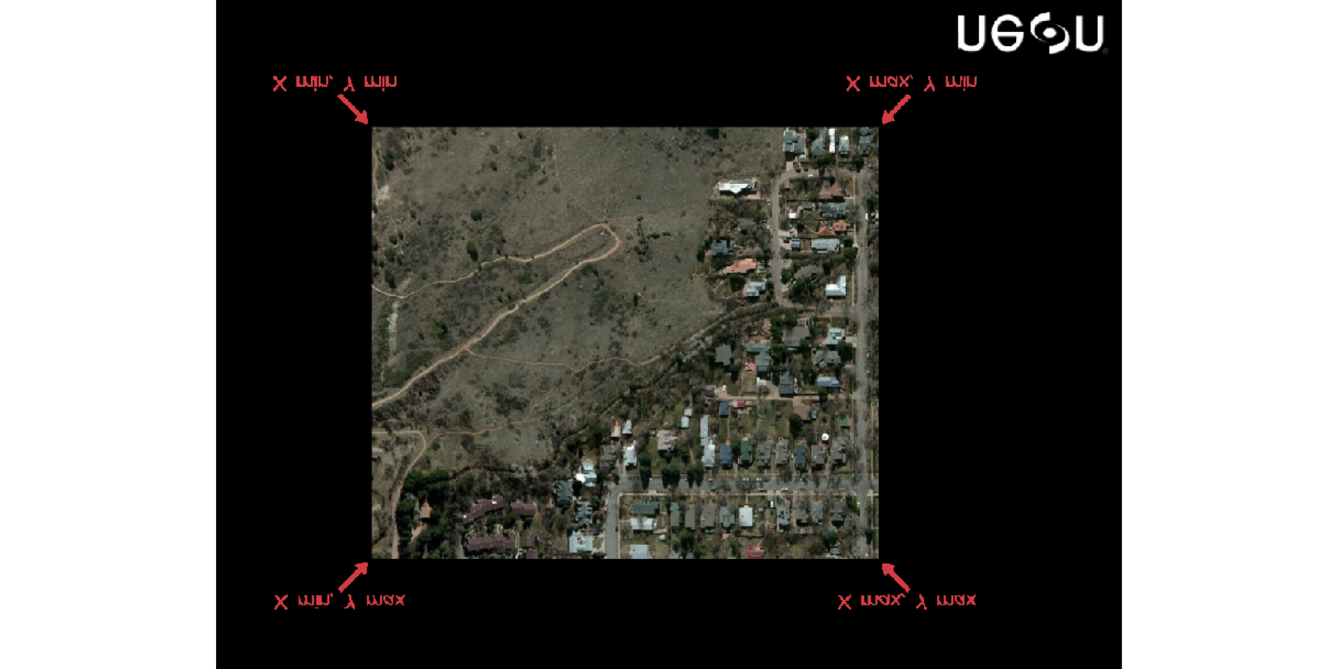
Assigning values as a vector
values(r) <- 1:ncell(r)

r
#> class       : SpatRaster
#> size        : 20, 20, 1  (nrow, ncol, nlyr)
#> resolution  : 2, 2  (x, y)
#> extent      : -120, -80, 20, 60  (xmin, xmax, ymin, ymax)
#> coord. ref. : lon/lat WGS 84 (CRS84) (OGC:CRS84)
#> source(s)   : memory
#> name        : lyr.1
#> min value   :     1
#> max value   :   400

head(values(r))
#>      lyr.1
#> [1,]     1
#> [2,]     2
#> [3,]     3
#> [4,]     4
#> [5,]     5
#> [6,]     6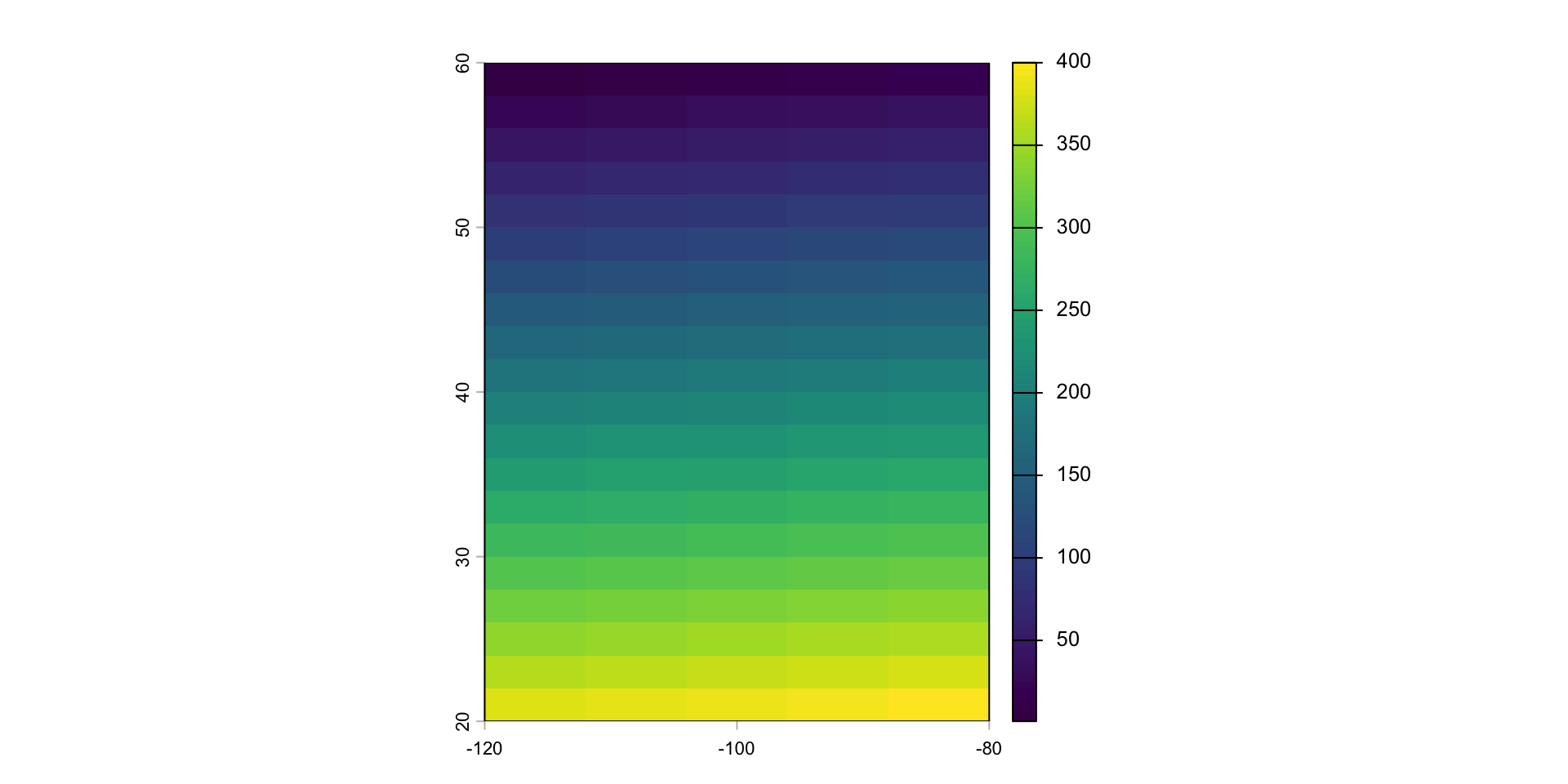
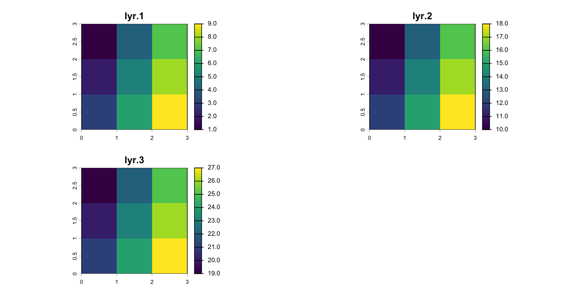
Multi-layers
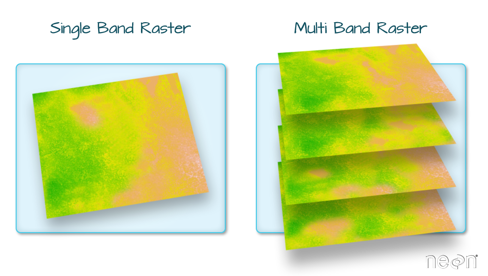
In many cases, multi-variable raster datasets are used. Variables can be related to time or measurement.
A SpatRaster is a collection of objects with the same spatial extent and resolution.
In essence it is a list of objects, or a 3D array.
An array is a single file so it can be “rasterized”
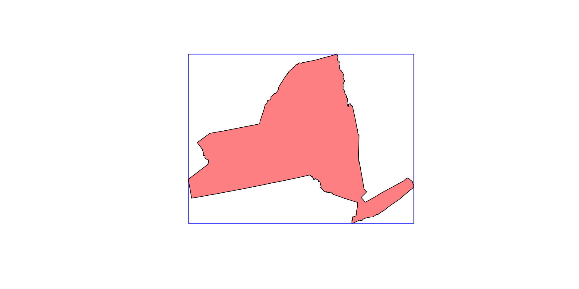
1. Bounding Box / Extents
Geometries have extents that define the maximum and minimum coverage of the shape in a coordinate reference system
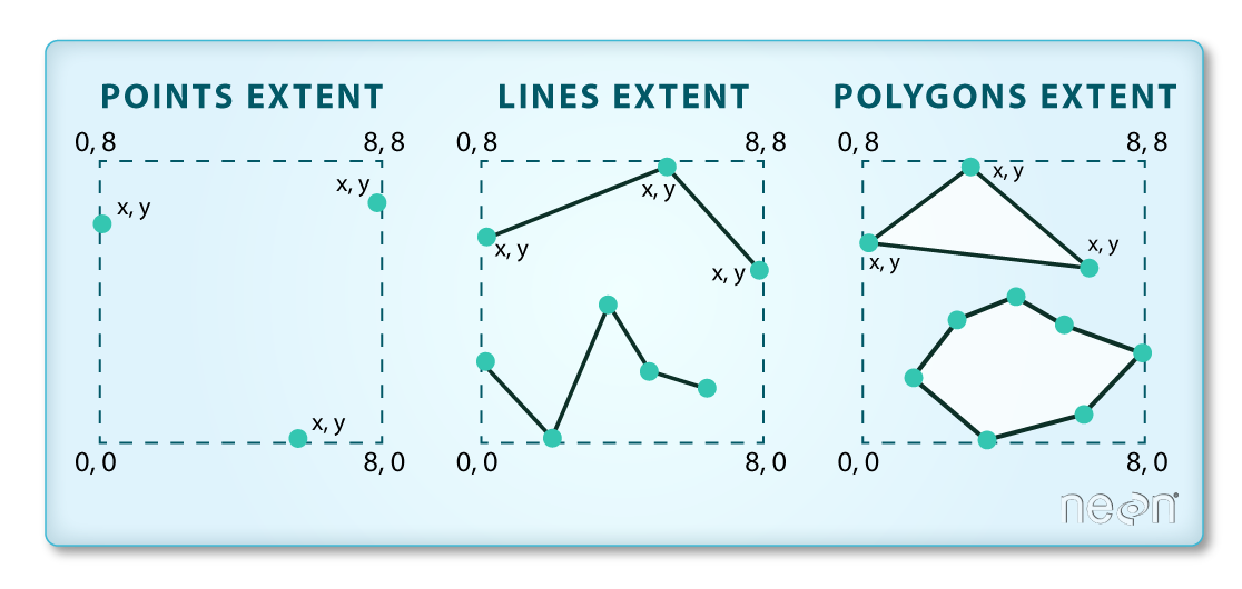
Image Source: National Ecological Observatory Network (NEON)
2. Extent
When dealing with objects, the extent (or bbox) is derived from the coordinate set
When dealing with raster data, the extent is a foundational component of the raster data structure
- That is, we need to know the area the raster is covering!
Image Source: National Ecological Observatory Network (NEON)
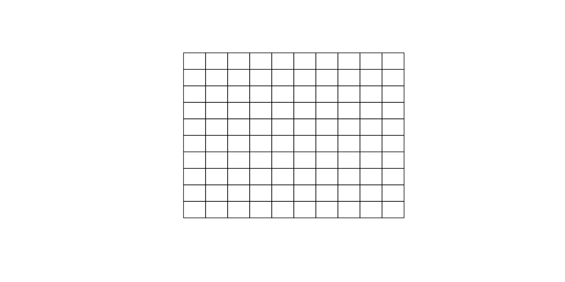
3. Discretization
Once we know the extent, we need to know how that space is split up
Two complementary pieces of information tell us this:
- Resolution (res)
- Number of row and number of columns (nrow/ncol)
Image Source: National Ecological Observatory Network (NEON)
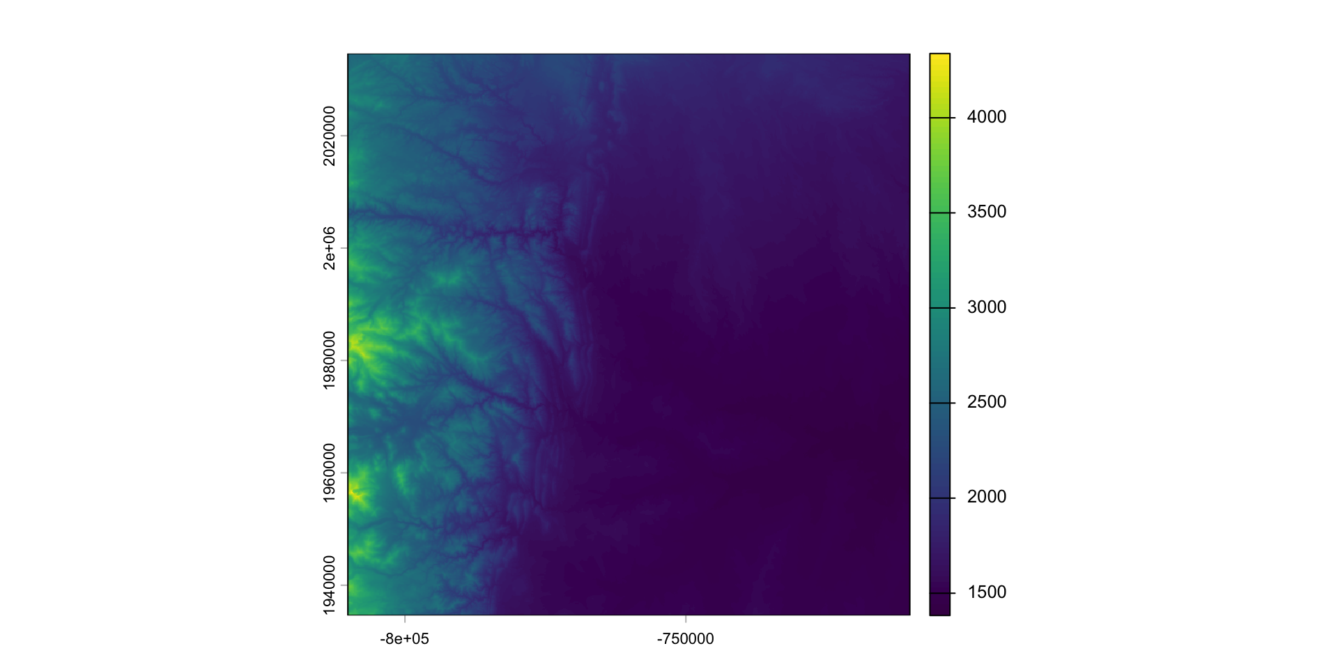
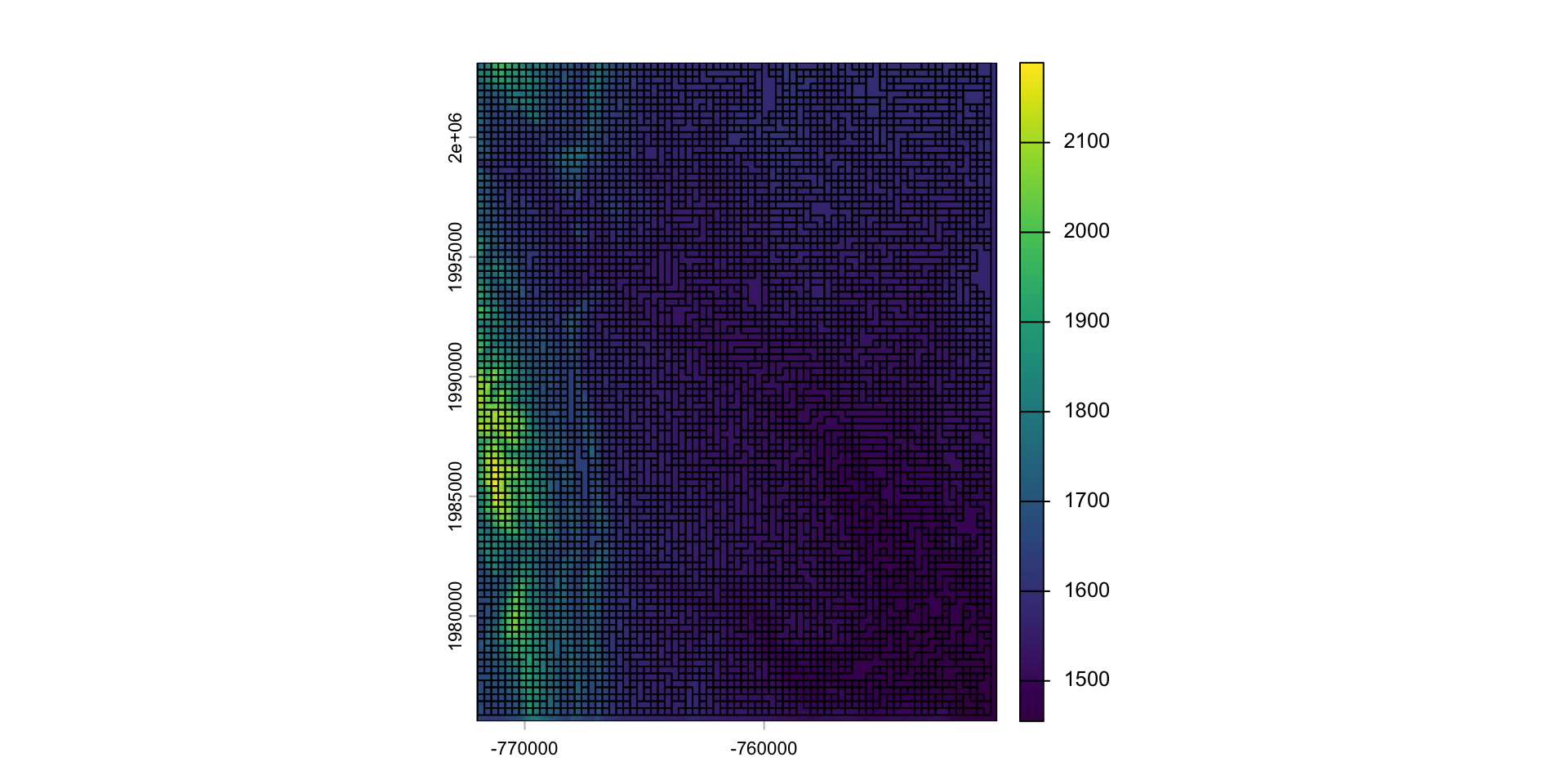
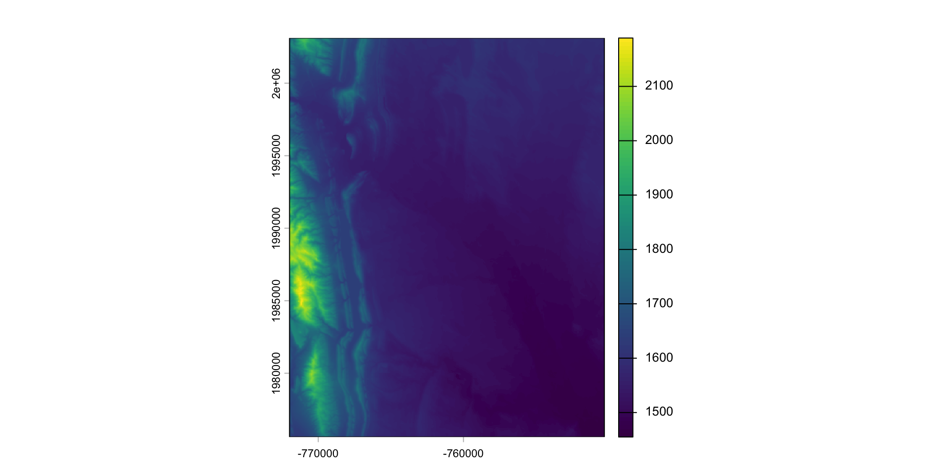
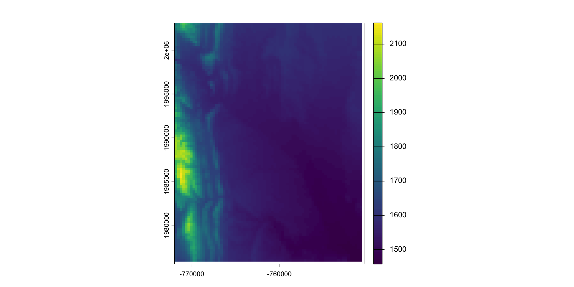
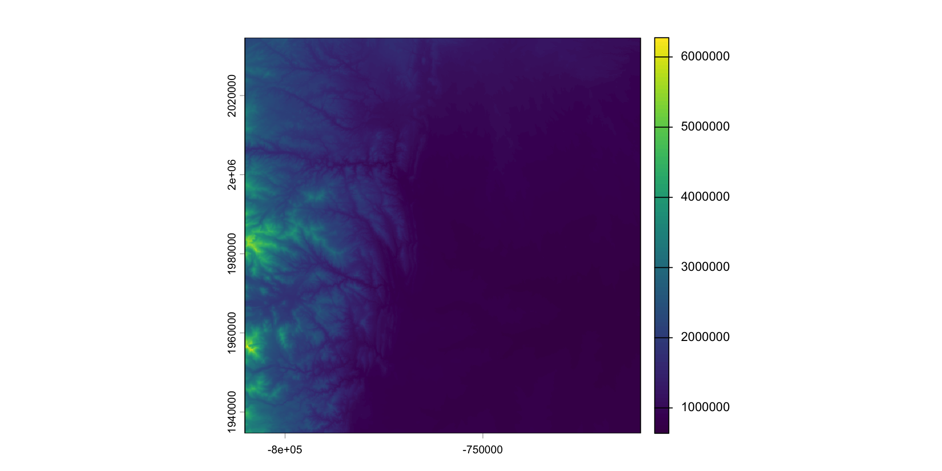
Find elevation data for Fort Collins:
- Define the AOI
- Read data from elevation map tiles, for a specific zoom, and crop to the AOI
- The resulting raster …
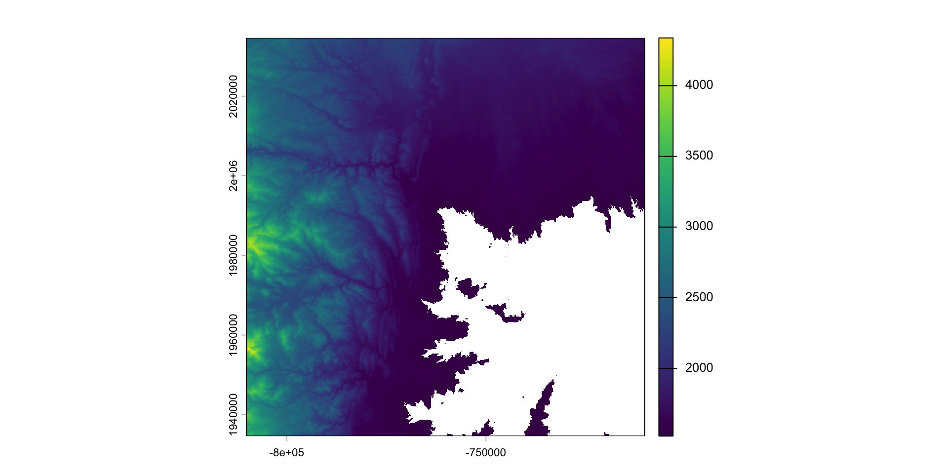
(elev = rast("data/foco-elev.tif"))
#> class       : SpatRaster
#> size        : 3450, 3450, 1  (nrow, ncol, nlyr)
#> resolution  : 28.98965, 28.98965  (x, y)
#> extent      : -810156.6, -710142.3, 1934613, 2034627  (xmin, xmax, ymin, ymax)
#> coord. ref. : +proj=aea +lat_0=23 +lon_0=-96 +lat_1=29.5 +lat_2=45.5 +x_0=0 +y_0=0 +datum=NAD83 +units=m +no_defs
#> source      : foco-elev.tif
#> name        : foco-elev
#> min value   :      1382
#> max value   :      4346
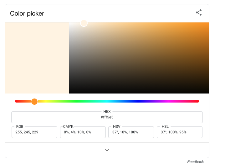
Google Color Picker
Replacement
- Raster values can be replaced using conditional statements
- Doing this changes the underlying data!
- If you want to retain the original data, you must make a copy of the base layer
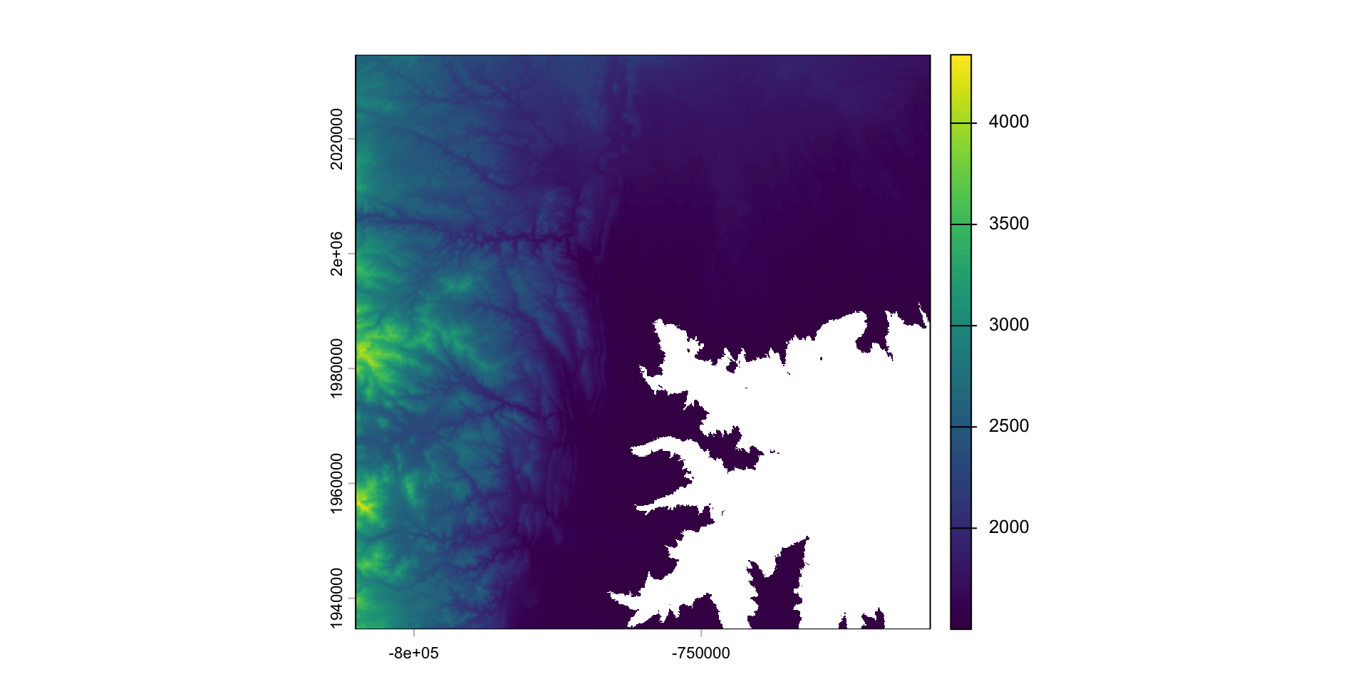
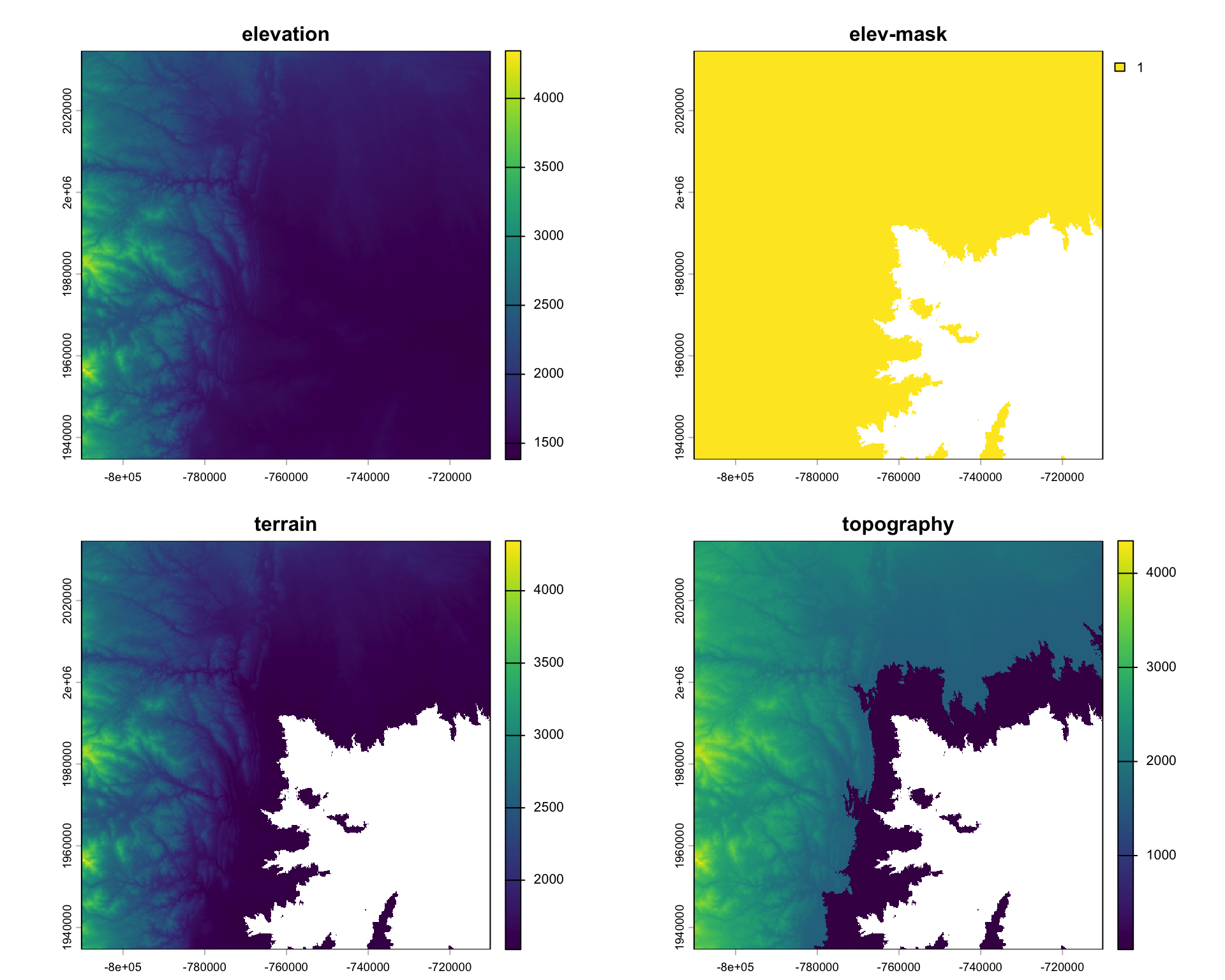
Modifying a raster
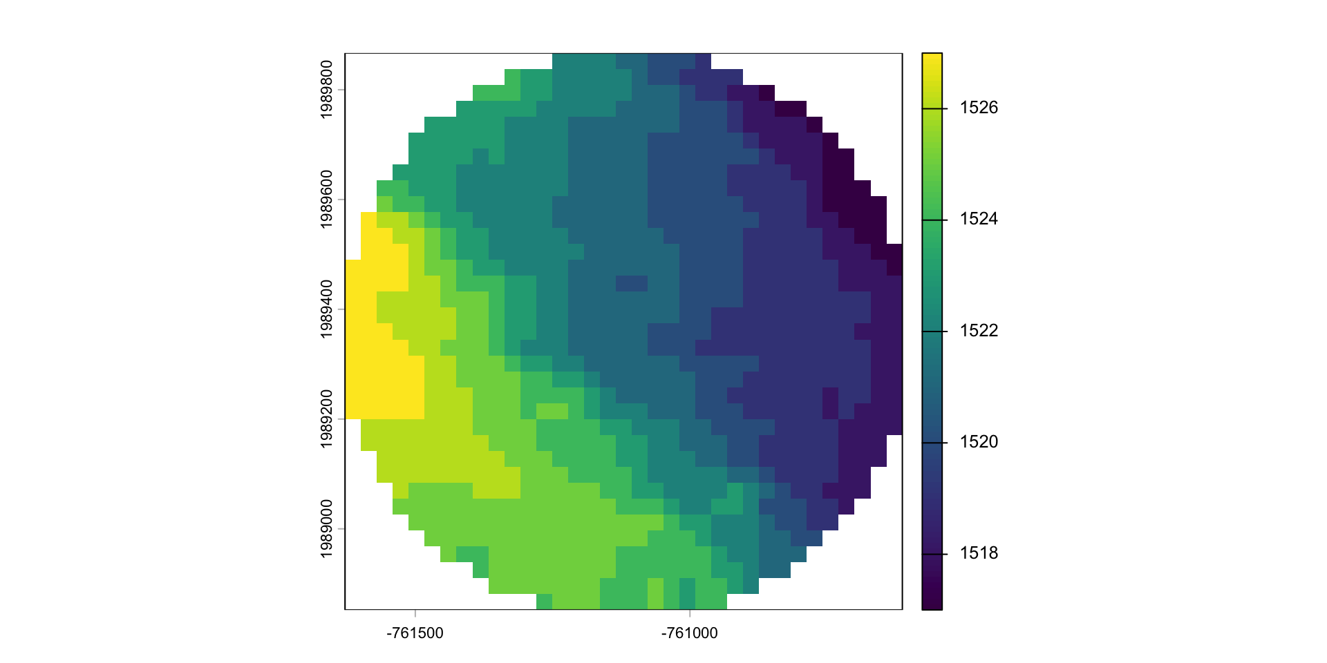
When we want to modify the extent of a raster we can clip it to a new bounds
crop: lets you reduce the extent of a raster to the extent of another, overlapping object:


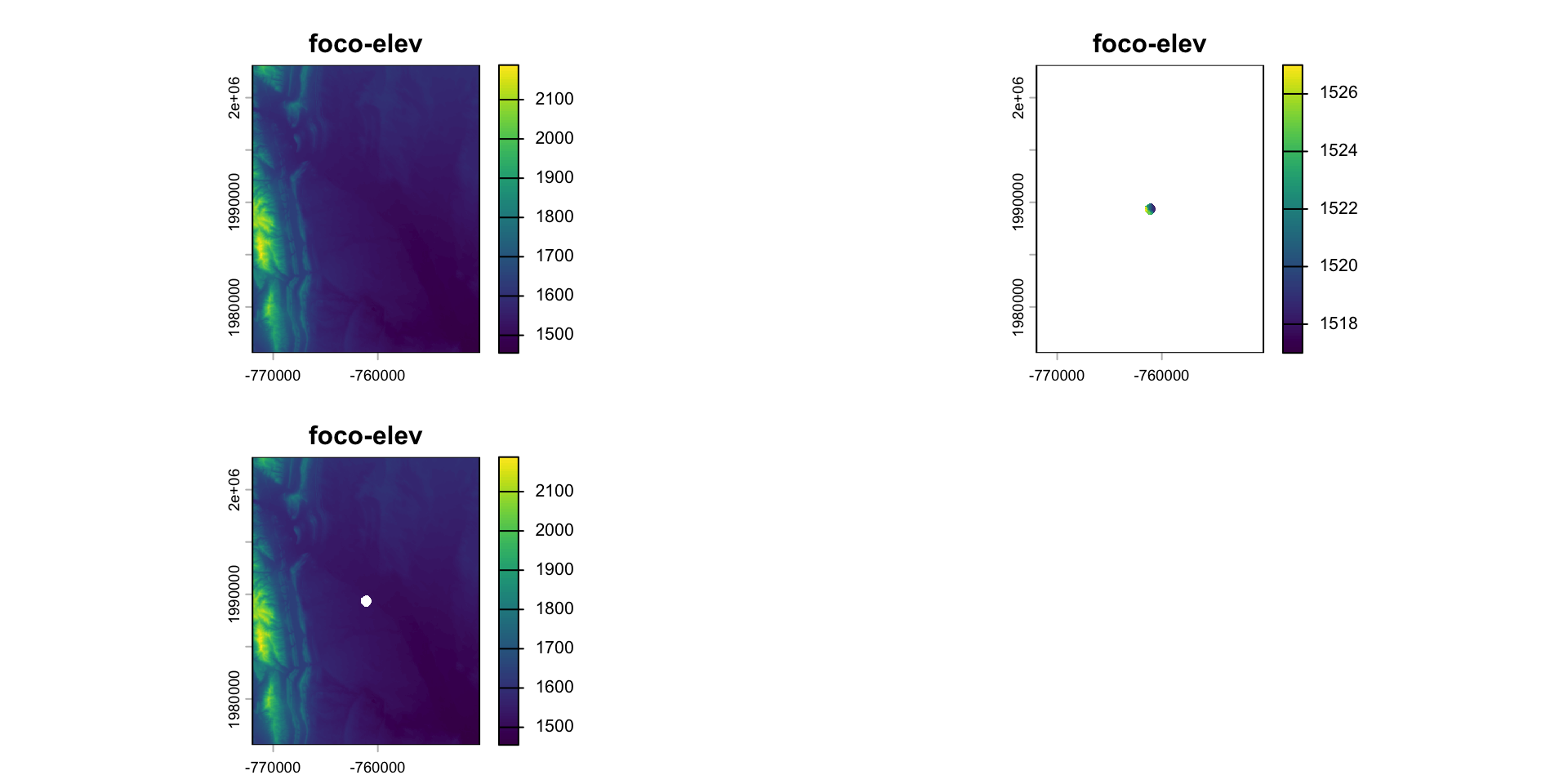
What is mask doing?
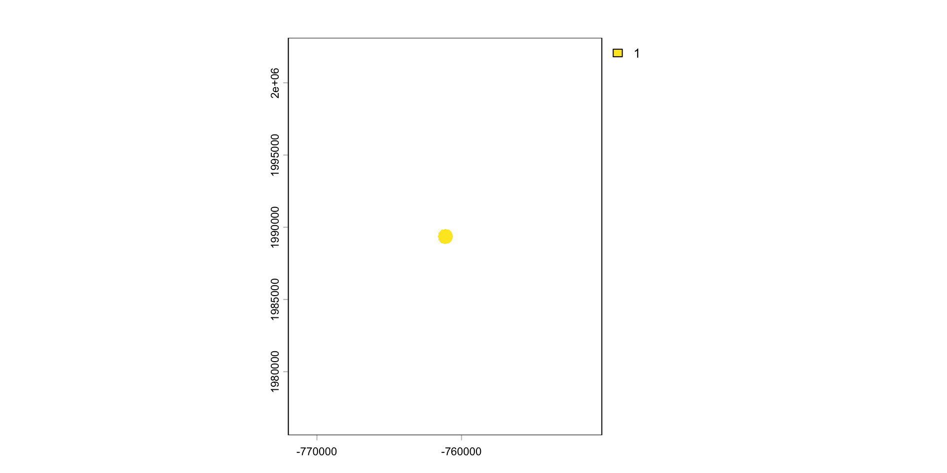
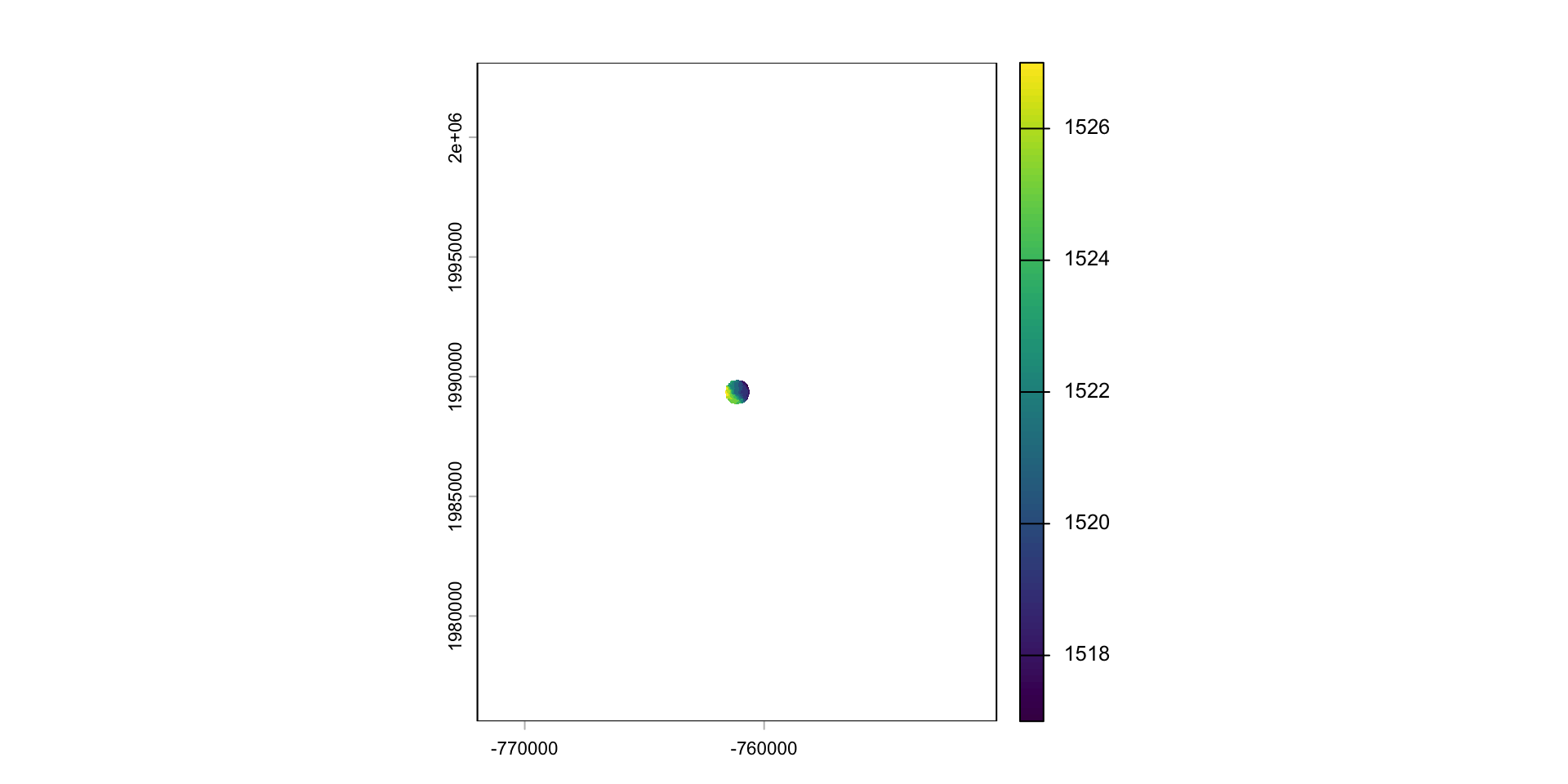
Crop or/and mask
- Crop is more efficient then mask
- Often you will want to mask and crop a raster
- The correct way to do this is crop then mask
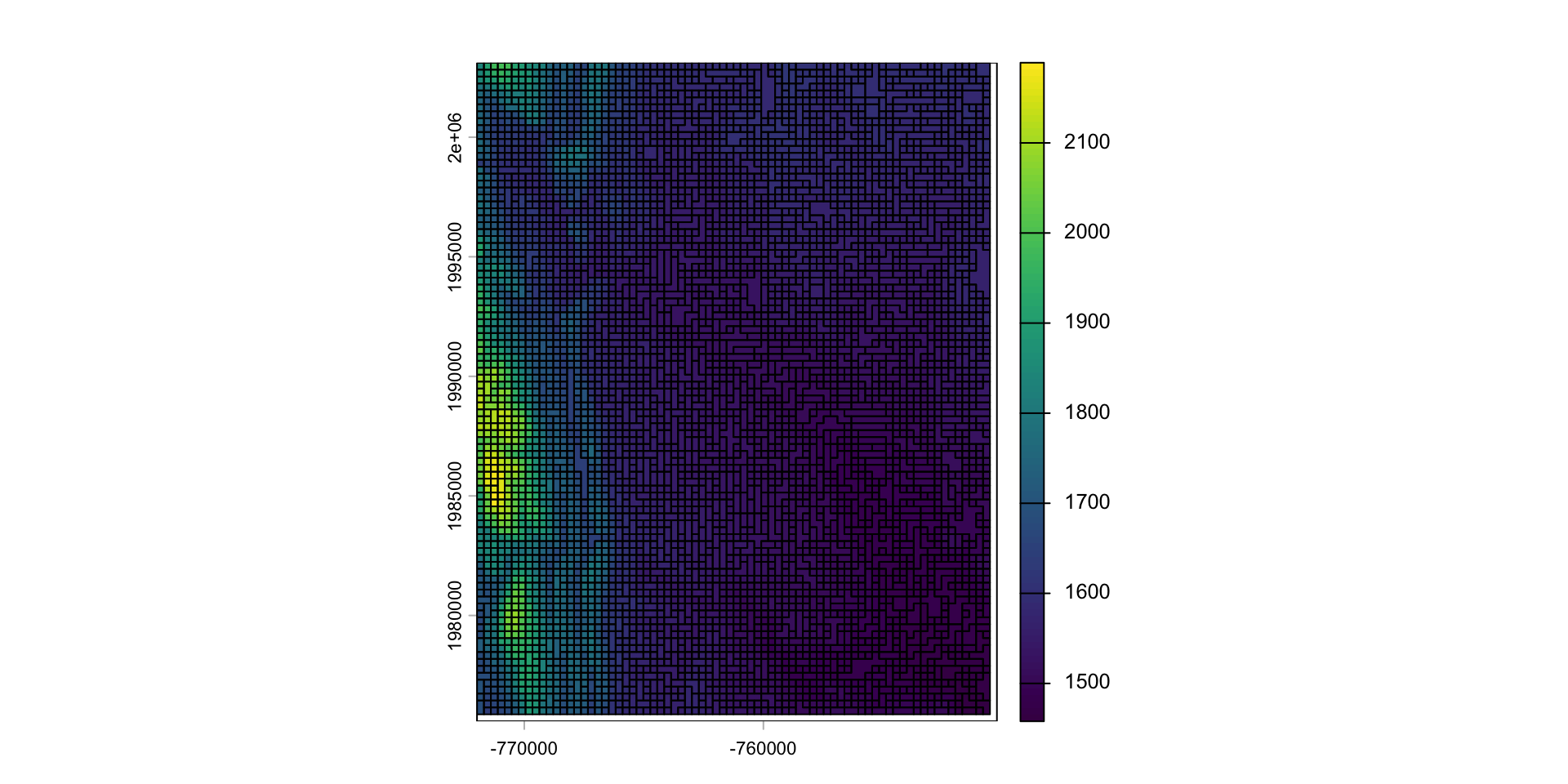
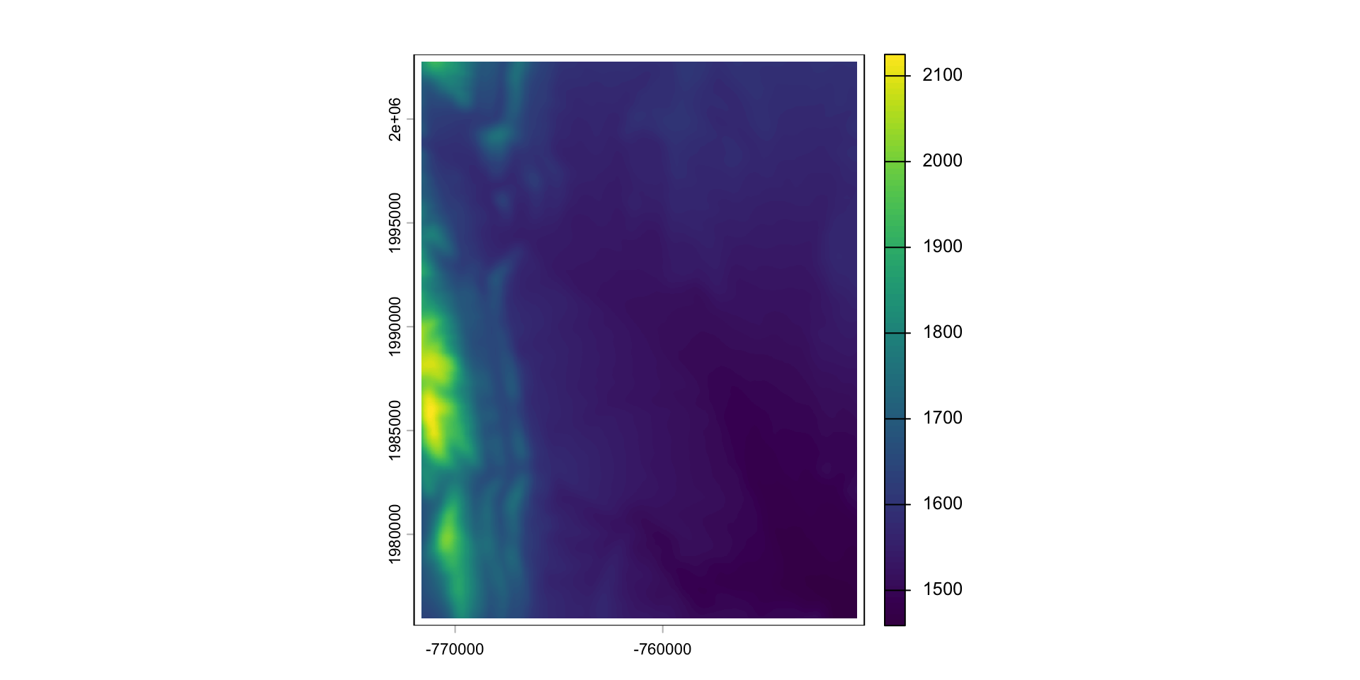
Aggregate and disaggregate
aggregateanddisaggregateallow for changing the resolution of a Raster object.This is similar to the zoom scaling on a web map except the scale factor is not set to 2
For aggregate, you need to specify a function determining what to do with the grouped cell values (default = mean).
app
Just like a vector, we can apply functions over a raster with app
These types of formulas are very useful for thresholding analysis
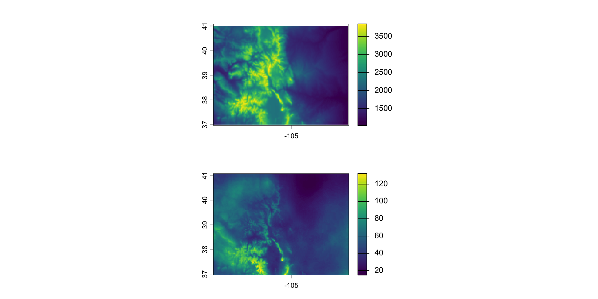
Question: separate Fort Collins into the higher and lower elevations
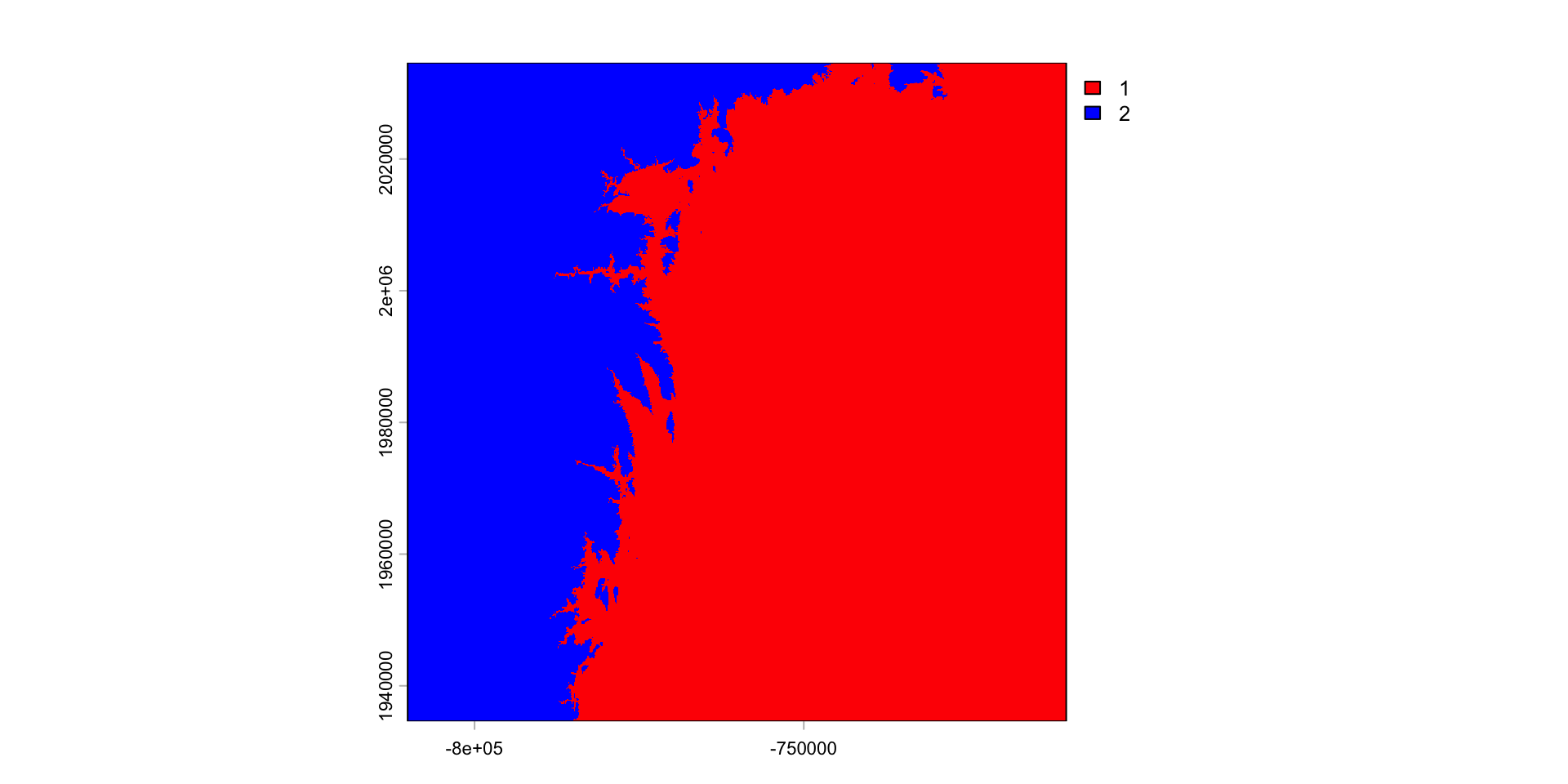
Results

Multiply cell-wise
- algebraic, logical, and functional operations act on a raster cell-wise
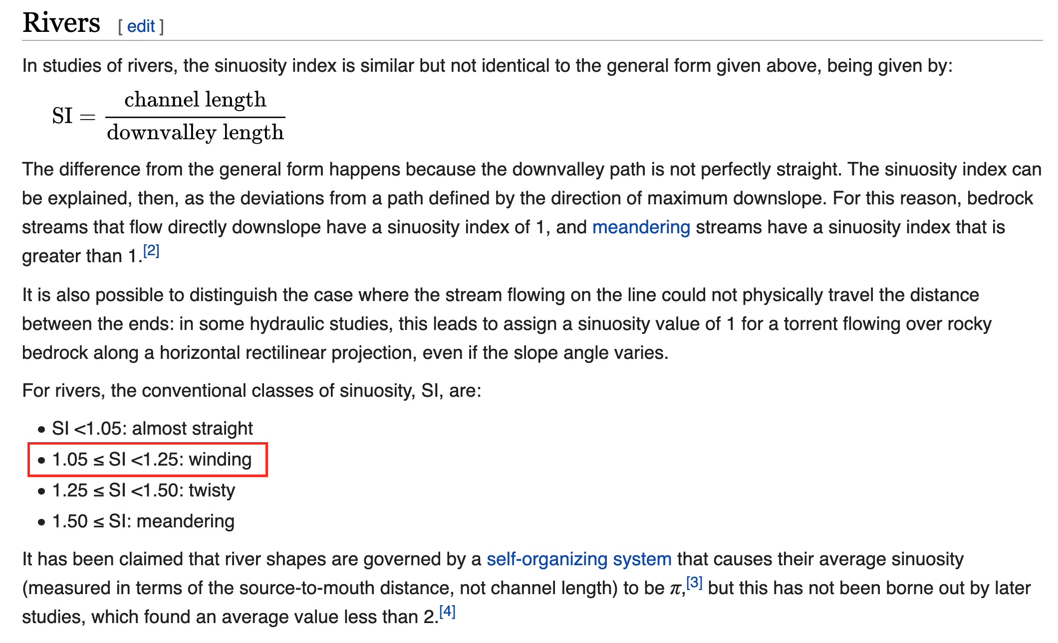
Lets find the longest river segment IN our extent


Sinuosity
Channel sinuosity is calculated by dividing the length of the stream channel by the straight line distance between the end points of the selected channel reach.
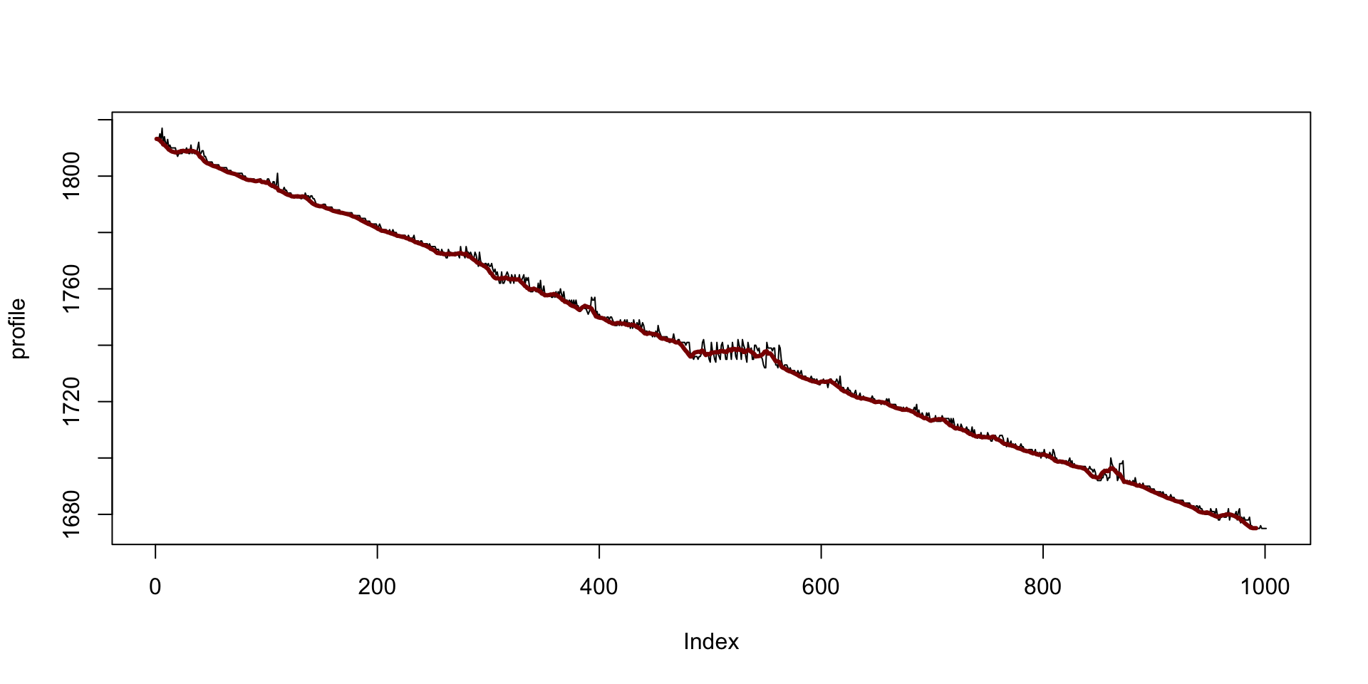
River profile
What does the elevation profile of the river look like?
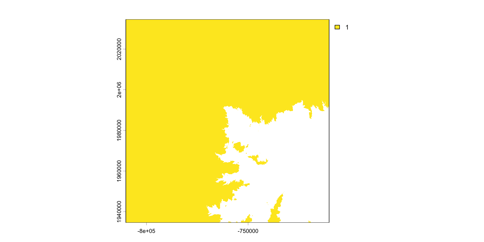
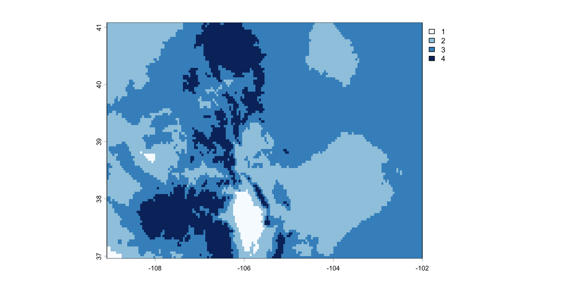
Local
Local operations and functions are applied to each individual cell and only involve those cells sharing the same location.
More than one raster can be involved in a local operation.
For example, rasters can be summed ( each overlapping pixels is added)
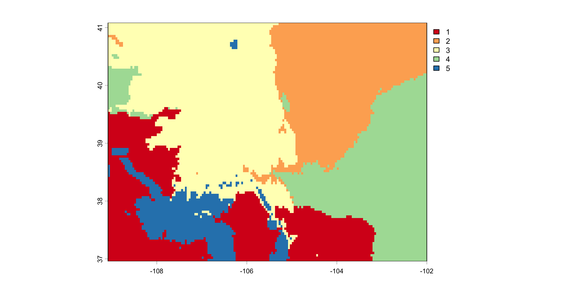
Local operations also include reclassification of values.
Results
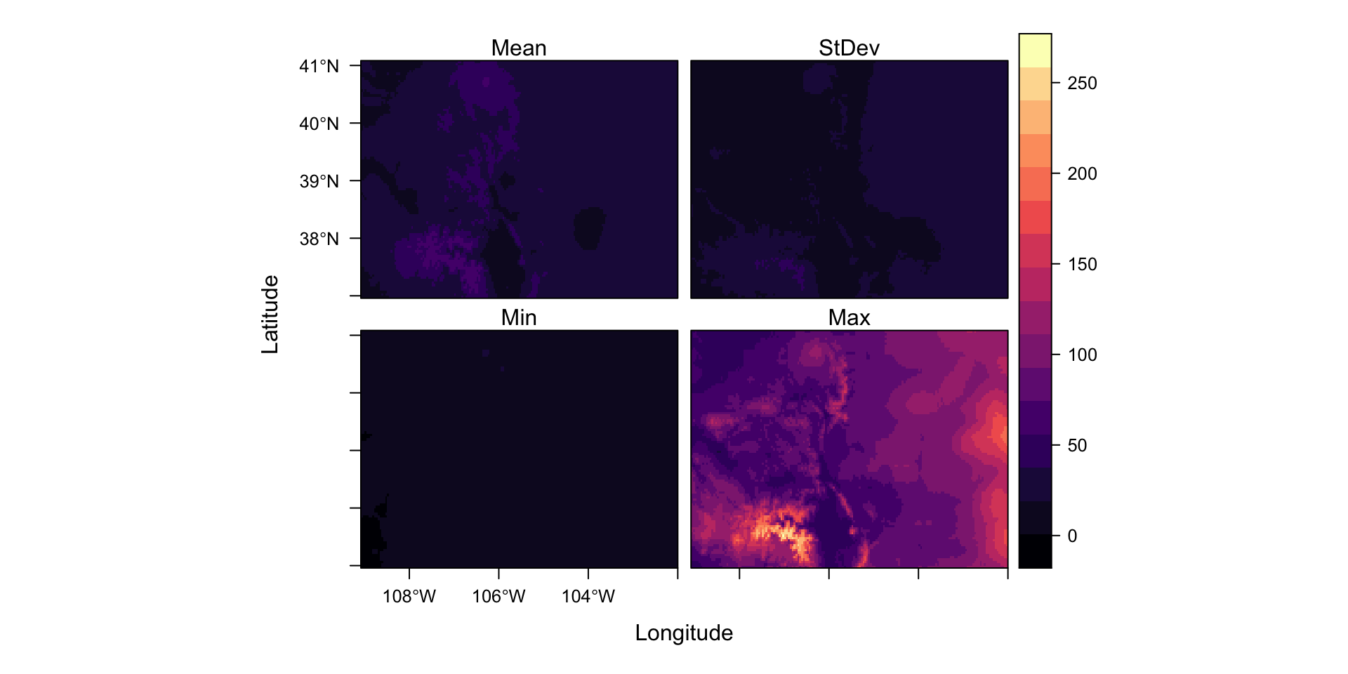
Zonal
Zonal operations compute a summary values (such as the mean) from cells aggregated to some zonal unit.
Like focal operations, a zone and a summary function must be defined
The most basis example of a zonal function is aggregation!
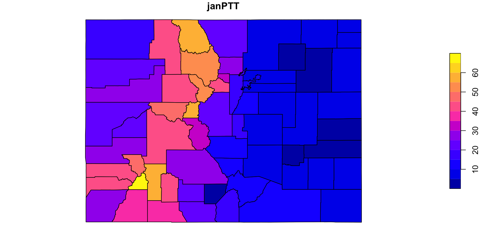
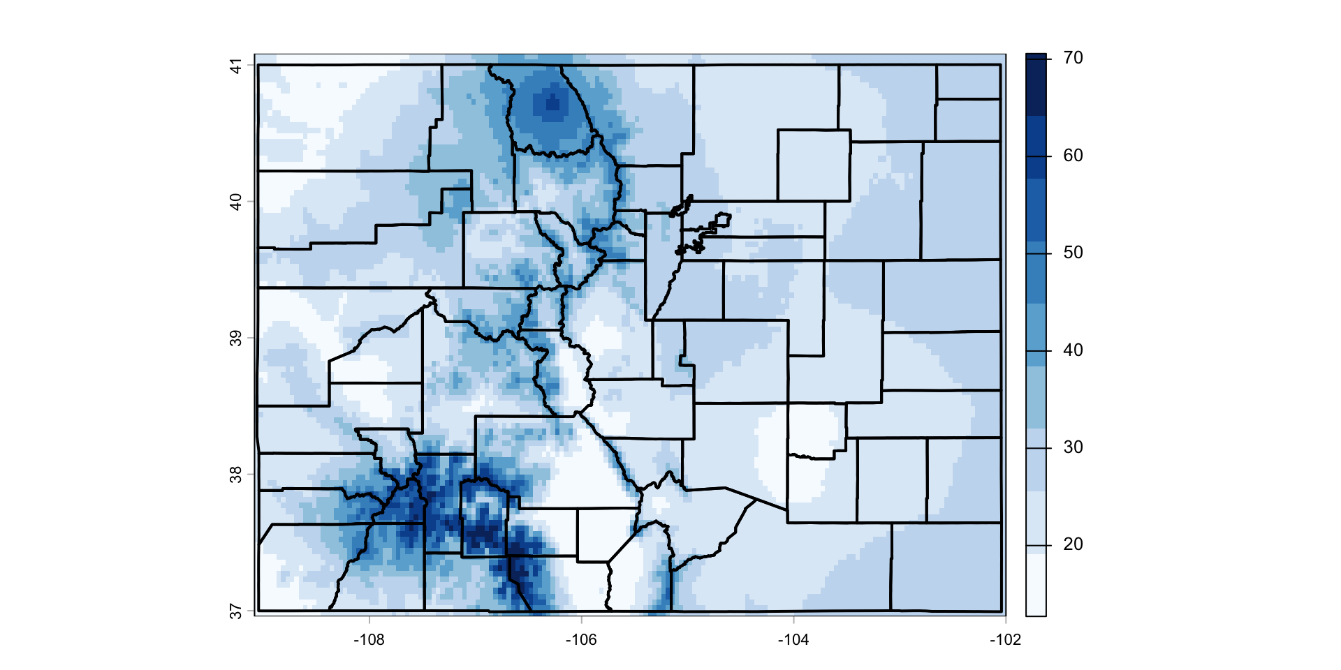
Zonal Statisics (More advanced)
For more complicated object zones, exactextractr is a fast and efficient R utility that binds the C++
exactextracttool.What is the county level mean January rainfall in Colorado?
Why not just mean()
In the terra package, functions like max, min, and mean, return a new SpatRast* object (with a value computed for each cell).
In contrast, global returns a single value, computed from the all the values of a layer.
Mean Monthly Rainfall for Colorado
global
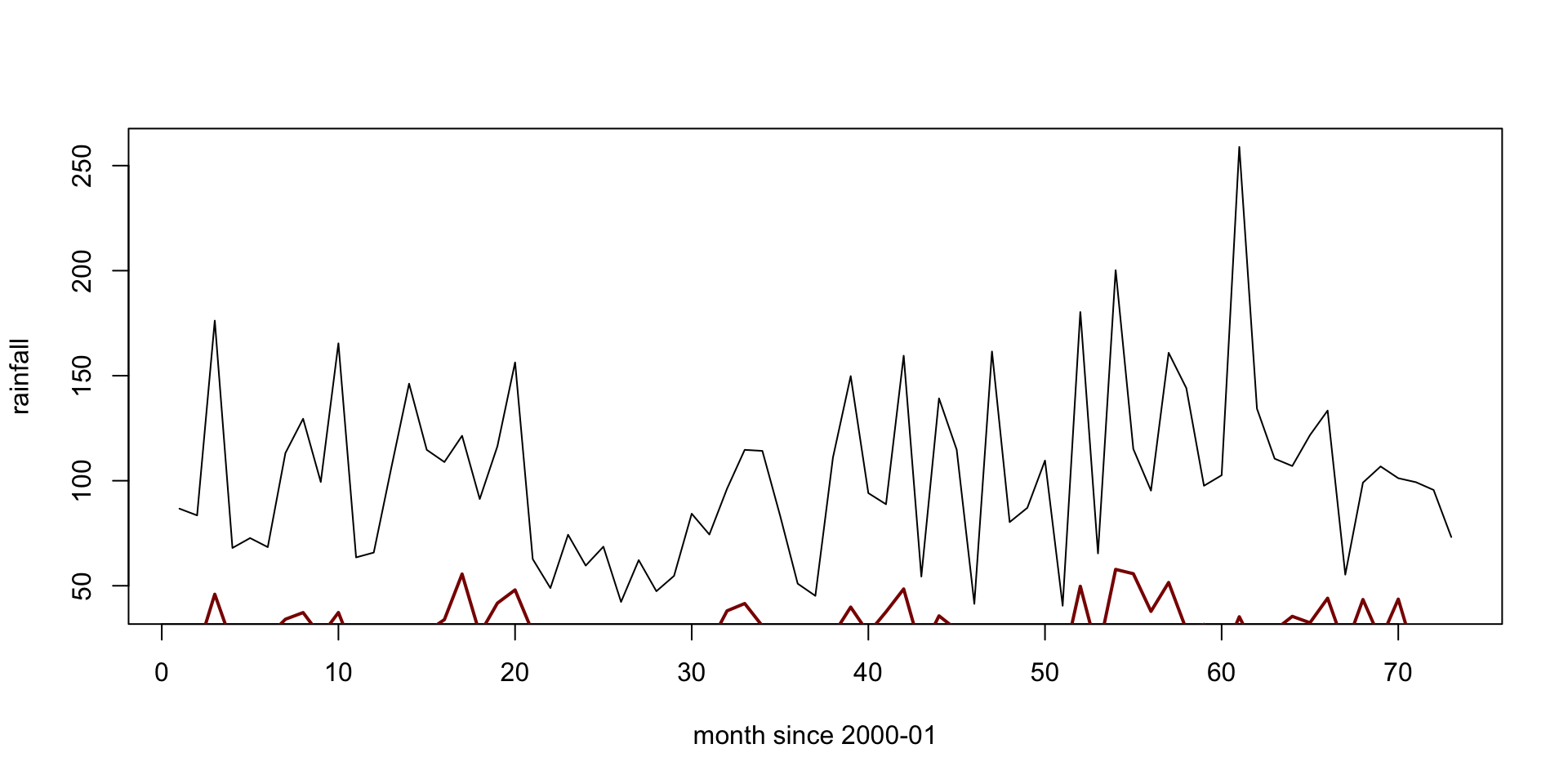
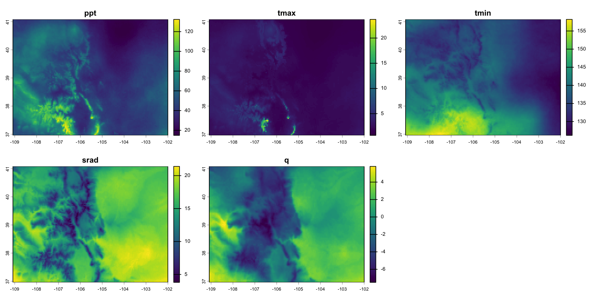
Colorado October 2018 climate
Assign values
Result