library(jsonlite)

# Parse JSON string
response_json <- '{"gauge":"Lees Ferry","flow":12400}'
(data <- fromJSON(response_json))
#> $gauge
#> [1] "Lees Ferry"
#>
#> $flow
#> [1] 12400

# Convert R object back to JSON
data_out <- toJSON(data, pretty = TRUE)
cat(data_out)
#> {
#>   "gauge": ["Lees Ferry"],
#>   "flow": [12400]
#> }Week 4-2
JSON, GeoJSON, and STAC: Cloud-Native Geospatial Discovery
Live Read
basin <- sf::read_sf('https://api.water.usgs.gov/nldi/linked-data/nwissite/USGS-11120000/basin')

basin
#> Simple feature collection with 1 feature and 0 fields
#> Geometry type: POLYGON
#> Dimension:     XY
#> Bounding box:  xmin: -119.8295 ymin: 34.41806 xmax: -119.7307 ymax: 34.52038
#> Geodetic CRS:  WGS 84
#> # A tibble: 1 × 1
#>                                                                         geometry
#>                                                                    <POLYGON [°]>
#> 1 ((-119.7732 34.43021, -119.7742 34.42717, -119.7832 34.42023, -119.8045 34.41…

plot(basin)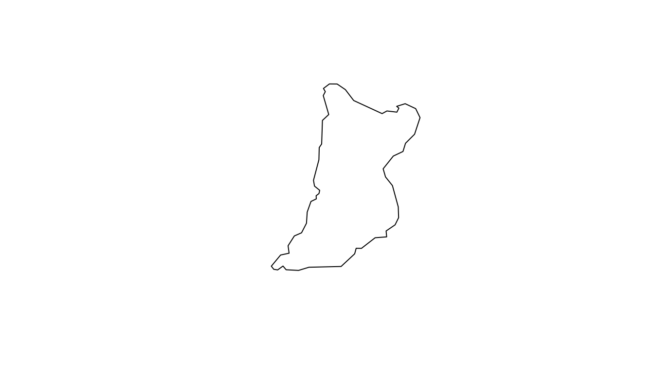
STAC Concepts
- Catalog: Describes a collection of data (e.g., Landsat Collection 2 Level-2)
- Collection: Metadata + spatial/temporal extent for a dataset
- Item: Single asset (one satellite scene), with its own metadata (cloud cover, datetime, bands)
- Asset: Specific file or data product (red band, NIR band, thumbnail, cloud mask)
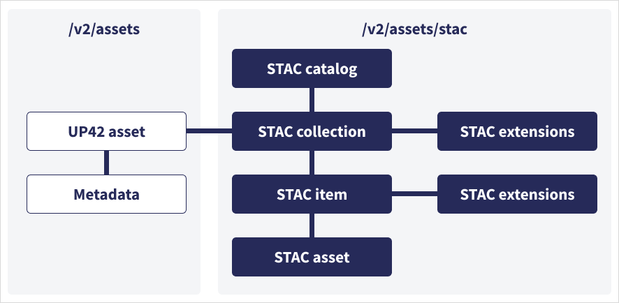
STAC hierarchy: Catalog → Collection → Item → Asset
Key insight: This nested structure lets you query at any level (find catalogs, browse collections, search for items, download specific assets).
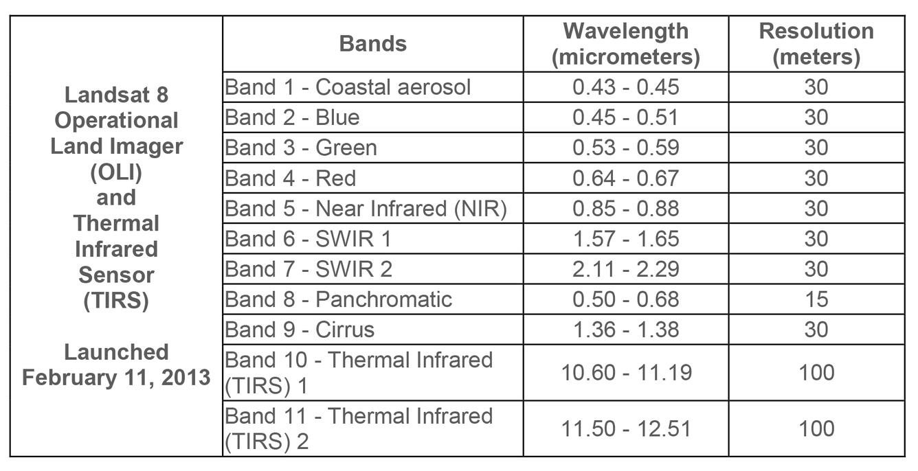
STAC Item Anatomy (Landsat Example)
{
  "type": "Feature",
  "id": "LC08_L2SP_025031_20160926_02_T1",
  "stac_version": "1.0.0",
  "geometry": { "type": "Polygon", "coordinates": [...] },
  "properties": {
    "datetime": "2016-09-26T16:47:00Z",
    "platform": "landsat-8",
    "instruments": ["OLI", "TIRS"],
    "eo:cloud_cover": 2.1
  },
  "assets": {
    "red": { "href": "s3://...LC08_red.TIF" },
    "nir": { "href": "s3://...LC08_nir.TIF" }
  }
}
Key insight: Assets are URLs pointing to cloud storage. A STAC item is essentially metadata + pointers to files.
Complete Walkthrough: Visualize Band Combinations
Natural Color (RGB) — What the Human Eye Would See
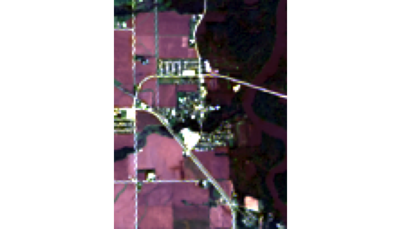
Visible: Water (dark), vegetation (green), urban (gray/tan), clouds (white)
Limitation: Flooding can look similar to vegetation in RGB alone.
Visualize: Color Infrared (Vegetation)
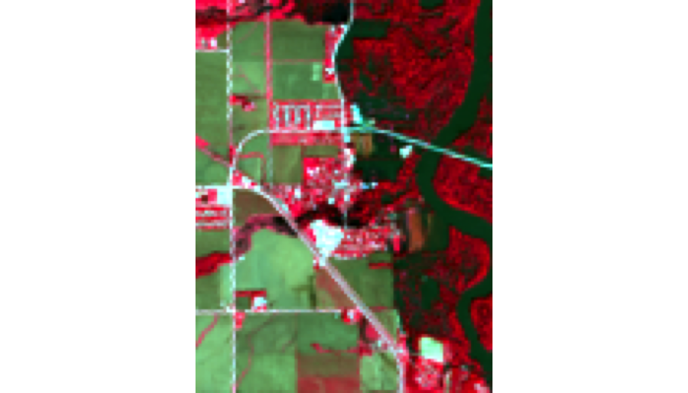
Visible: - Bright red/magenta = healthy vegetation (strong NIR reflectance) - Dark blue/black = water - Gray/tan = soil/urban
Why NIR matters: Vegetation reflects ~50% of NIR light; water absorbs it. This makes forests “glow” red.
Visualize: Water-Focused False Color
plotRGB(landsat_crop, r = 5, g = 6, b = 4, stretch = "lin",
        main = "Water Focus: NIR-SWIR1-Red\n(Dark blue = open water/flooding)")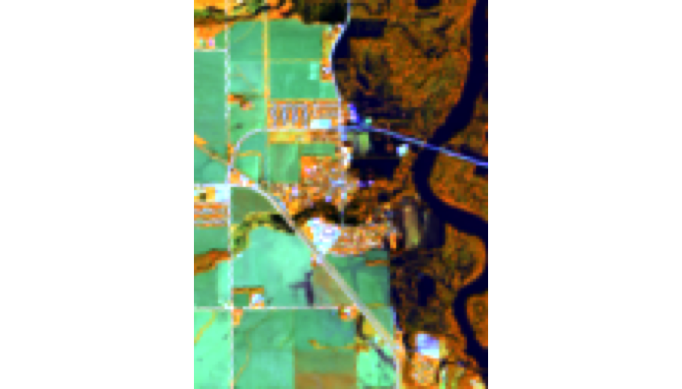
Visible: - Dark blue/black = open water, flooded areas (absorbs NIR + SWIR) - Bright colors = vegetation & land - Often shows flooding more clearly than natural color
Why SWIR1 matters: Water absorbs SWIR; vegetation reflects it. This combo best delineates water boundaries.

Complete Walkthrough: NDVI
$ NDVI = $
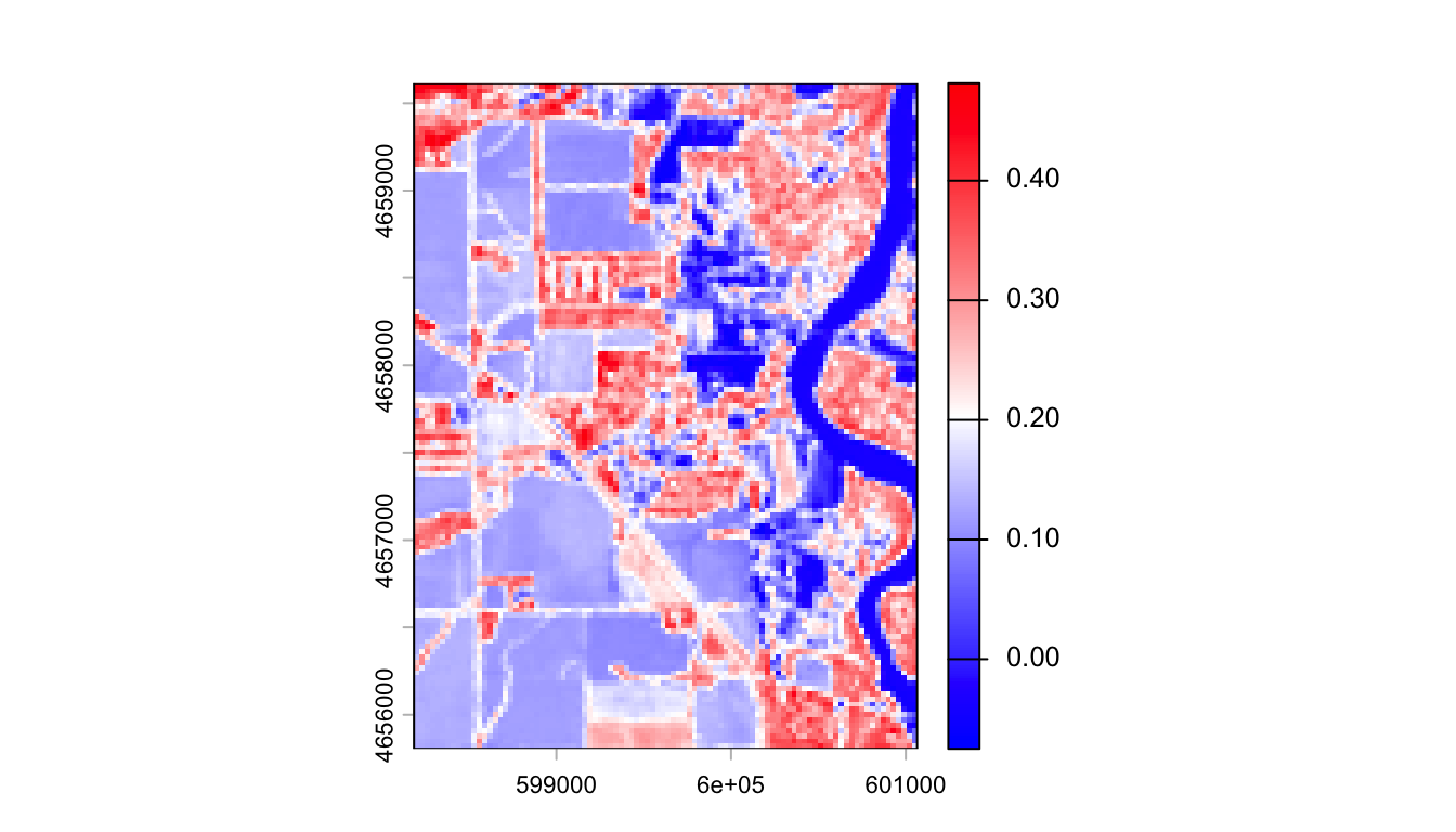
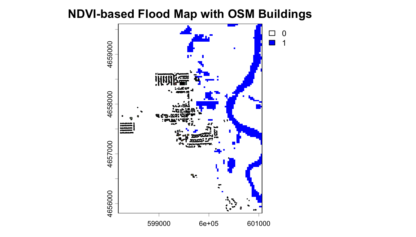
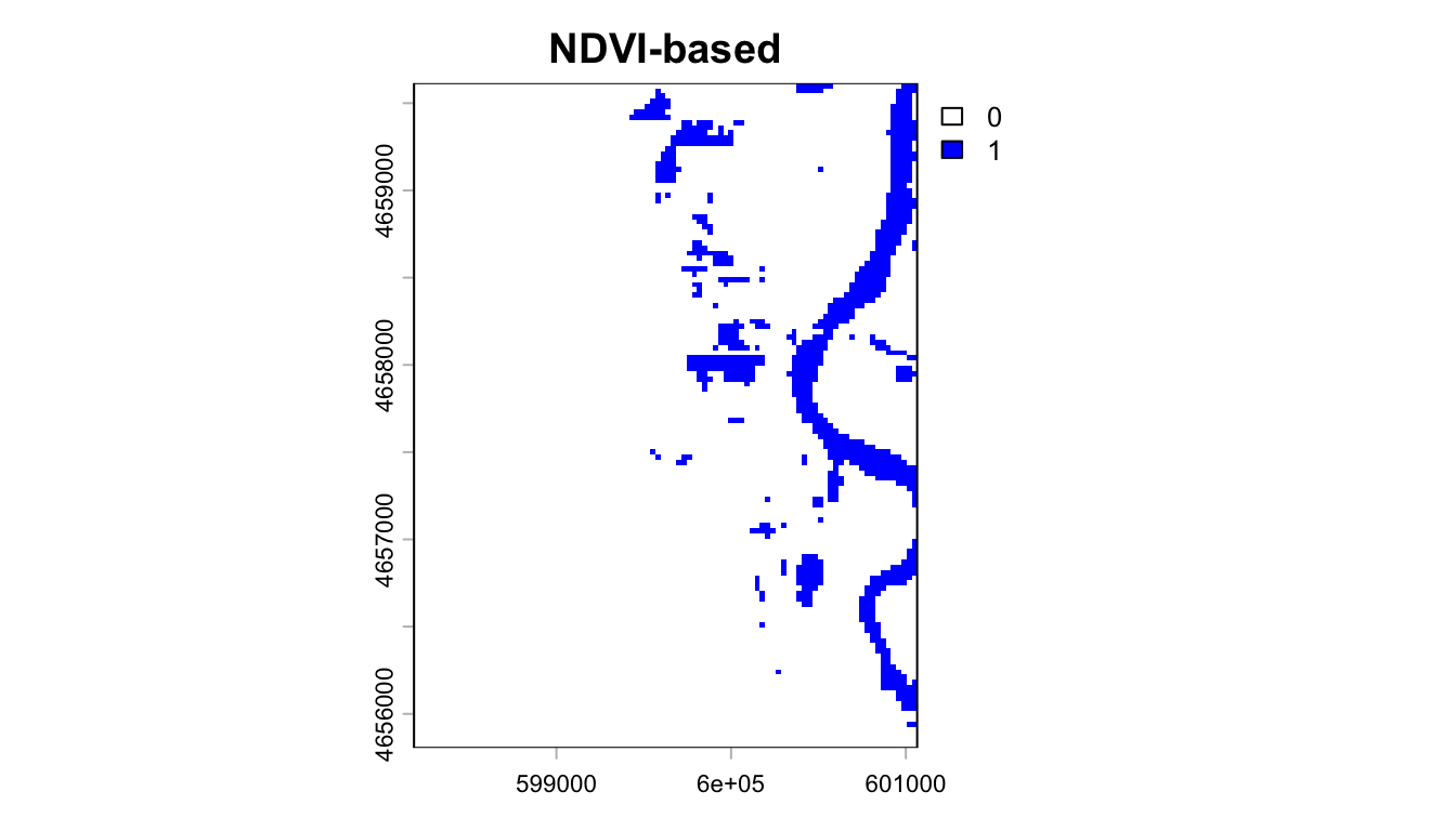
Thresholding to Binary Flood Maps
NDVI < 0 typically indicates water. We can apply this threshold to create a binary flood map:
Imapct Assessment: