Week 5

Machine Learning Part 1

Modeling (Machine Learning)

By the end of today you will be able to…

• Summarize a dataset’s structure and distributions using EDA tools (skimr, ggpubr, visdat)
• Assess whether data meets normality assumptions and choose an appropriate response (transform, nonparametric, bootstrap)
• Explain the role of training, testing, and resampling splits in a modeling workflow
• Specify a model with parsnip by choosing a type, engine, and mode
• Fit a model inside a workflow and evaluate it with yardstick metrics
• Compare multiple models at once with workflow_sets over cross-validation folds

Today’s running example: “Can we predict whether a 6,000-acre hexagon in Washington is forested?”

What is machine learning?

What is machine learning? (2025 edition)

Note

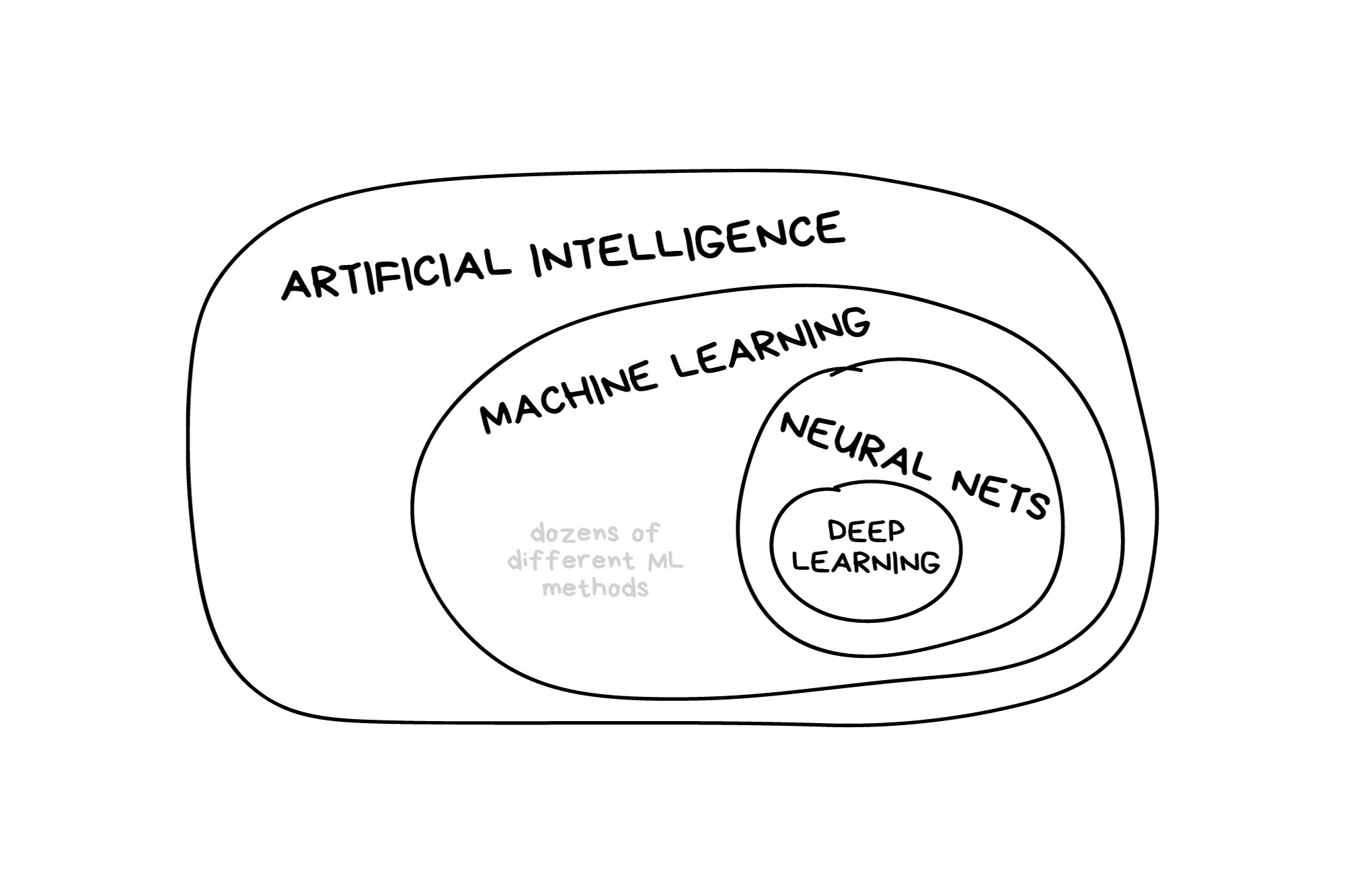
In the early 2010s, “Artificial intelligence” (AI) was largely synonymous with what we’ll refer to as “machine learning” in this workshop. In the late 2010s and early 2020s, AI usually referred to deep learning methods. Since the release of ChatGPT in late 2022, “AI” has come to also encompass large language models (LLMs) / generative models.

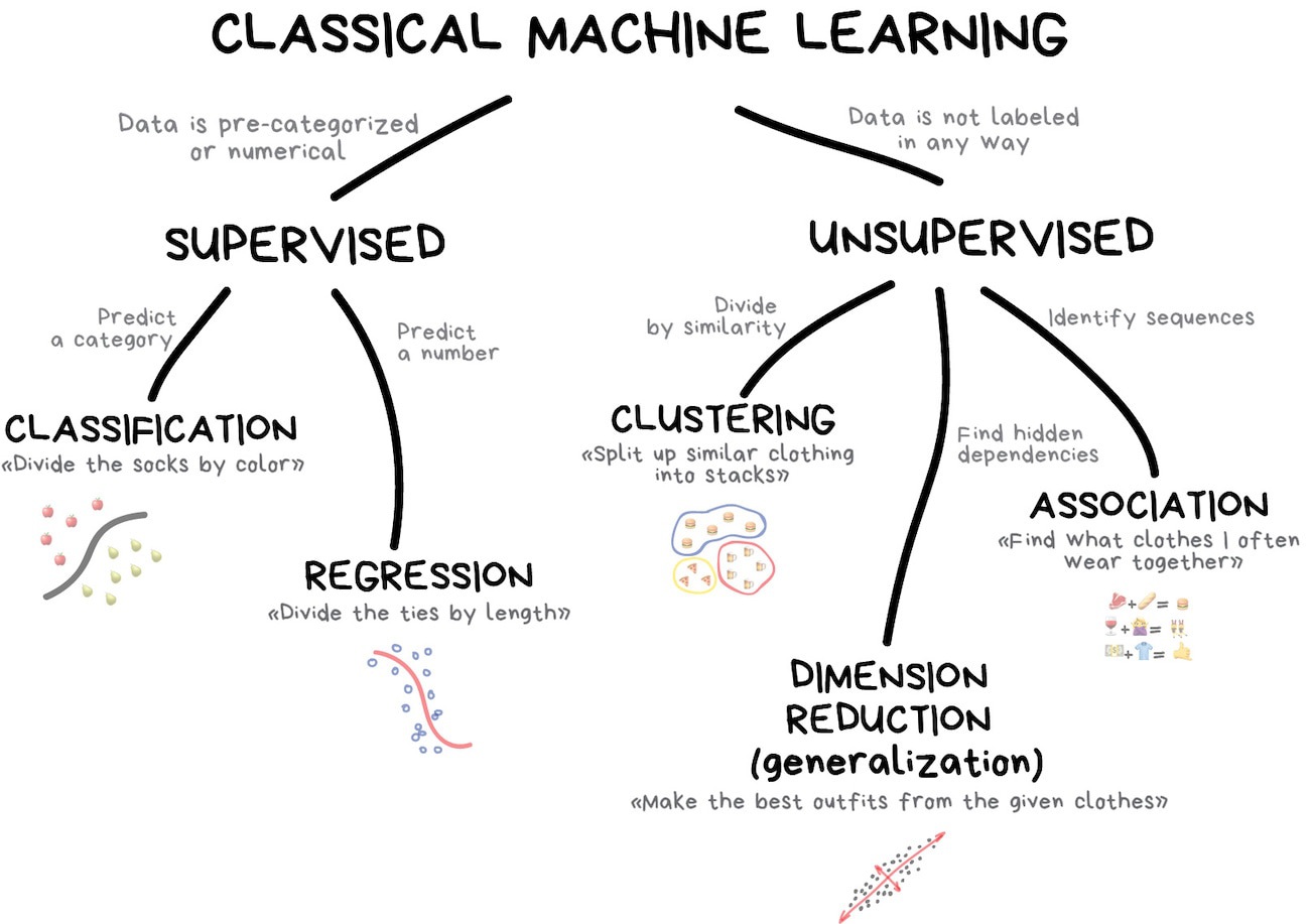
Classic Conceptual Model

The big picture: Road map

What is tidymodels?

• An R package ecosystem for modeling and machine learning
• Built on the tidyverse principles (consistent syntax, modular design)
• Provides a structured workflow for preprocessing, model fitting, and evaluation
• Includes packages for model specification, preprocessing, resampling, tuning, and evaluation
• Promotes best practices for reproducibility and efficiency
• Offers a unified interface for different models and tasks

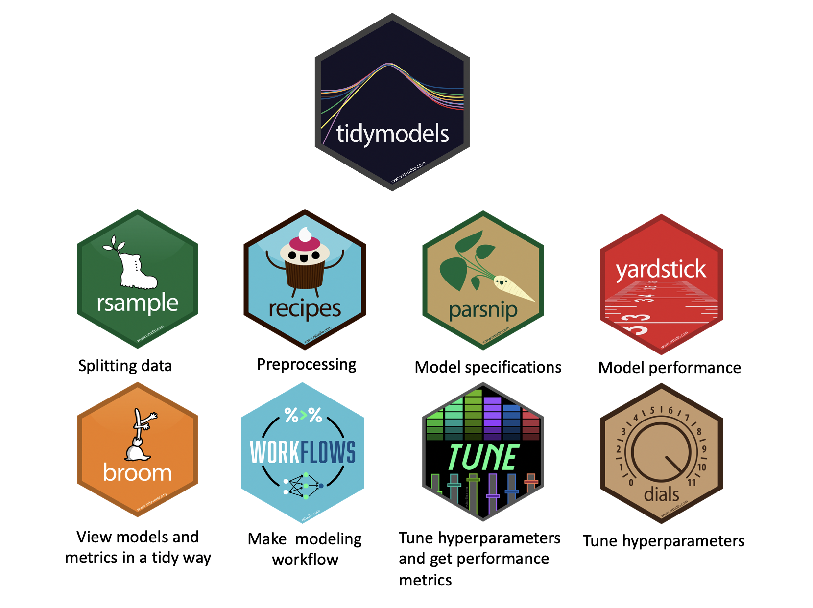
Key tidymodels Packages

📦 recipes: Feature engineering and preprocessing

📦 parsnip: Unified interface for model specification

📦 workflows: Streamlined modeling pipelines

📦 tune: Hyperparameter tuning

📦 rsample: Resampling and validation

📦 yardstick: Model evaluation metrics

knitr::include_graphics('img/tidymodels-packages.png')

tidymodels::tidymodels_packages()
#>  [1] "broom"        "cli"          "conflicted"   "dials"        "dplyr"       
#>  [6] "ggplot2"      "hardhat"      "infer"        "modeldata"    "parsnip"     
#> [11] "purrr"        "recipes"      "rlang"        "rsample"      "rstudioapi"  
#> [16] "tailor"       "tidyr"        "tune"         "workflows"    "workflowsets"
#> [21] "yardstick"    "tidymodels"

Typical Workflow in tidymodels

1️⃣ Load Package & Data

2️⃣ Preprocess Data (recipes)

3️⃣ Define Model (parsnip)

4️⃣ Create a Workflow (workflows)

5️⃣ Train & Tune (tune)

6️⃣ Evaluate Performance (yardstick)

Recap: lm() in R

You’ve used lm() before — this slide frames it as the foundation for everything broom and tidymodels build on top of.

lm() fits a linear model by ordinary least squares.

model <- lm(y ~ x1 + x2, data = df)

Key arguments:

• formula — response ~ predictors (. = all columns)
• data — the training data frame

Common follow-up functions:

Function	What it returns
summary(model)	Coefficients, R², F-statistic
coef(model)	Named coefficient vector
fitted(model)	In-sample predictions
residuals(model)	Raw residuals

mod <- lm(body_mass_g ~ bill_length_mm + species,
          data = drop_na(penguins))
summary(mod)
#> 
#> Call:
#> lm(formula = body_mass_g ~ bill_length_mm + species, data = drop_na(penguins))
#> 
#> Residuals:
#>     Min      1Q  Median      3Q     Max 
#> -860.77 -244.79    4.36  215.73 1075.25 
#> 
#> Coefficients:
#>                  Estimate Std. Error t value Pr(>|t|)    
#> (Intercept)       200.453    271.646   0.738    0.461    
#> bill_length_mm     90.298      6.951  12.991  < 2e-16 ***
#> speciesChinstrap -876.942     88.744  -9.882  < 2e-16 ***
#> speciesGentoo     596.702     76.429   7.807 7.88e-14 ***
#> ---
#> Signif. codes:  0 '***' 0.001 '**' 0.01 '*' 0.05 '.' 0.1 ' ' 1
#> 
#> Residual standard error: 375.2 on 329 degrees of freedom
#> Multiple R-squared:  0.7848, Adjusted R-squared:  0.7829 
#> F-statistic:   400 on 3 and 329 DF,  p-value: < 2.2e-16

Reading the output:

• Estimate — change in y per 1-unit increase in x
• Pr(>|t|) — p-value: is the coefficient ≠ 0?
• Adjusted R² — proportion of variance explained
• F-statistic — overall model significance

→ broom wraps this into tidy tibbles (next slide)

Recap: broom — tidying model outputs

broom converts messy model objects into tidy tibbles. Three core functions:

Function	Returns	Use it when you want to …
tidy()	One row per model term	Inspect coefficients, p-values, confidence intervals
glance()	One row per model	Compare overall fit (R², AIC, log-likelihood, …)
augment()	One row per observation	Add predictions, residuals, influence stats to data

simple_mod <- lm(body_mass_g ~ bill_length_mm + species, data = drop_na(penguins))

tidy(simple_mod)      # coefficients table
#> # A tibble: 4 × 5
#>   term             estimate std.error statistic  p.value
#>   <chr>               <dbl>     <dbl>     <dbl>    <dbl>
#> 1 (Intercept)         200.     272.       0.738 4.61e- 1
#> 2 bill_length_mm       90.3      6.95    13.0   1.97e-31
#> 3 speciesChinstrap   -877.      88.7     -9.88  2.46e-20
#> 4 speciesGentoo       597.      76.4      7.81  7.88e-14

Recap: broom in practice

glance(simple_mod)    # model-level fit statistics
#> # A tibble: 1 × 12
#>   r.squared adj.r.squared sigma statistic   p.value    df logLik   AIC   BIC
#>       <dbl>         <dbl> <dbl>     <dbl>     <dbl> <dbl>  <dbl> <dbl> <dbl>
#> 1     0.785         0.783  375.      400. 2.22e-109     3 -2444. 4899. 4918.
#> # ℹ 3 more variables: deviance <dbl>, df.residual <int>, nobs <int>

augment(simple_mod) |>
  select(body_mass_g, .fitted, .resid) |>
  head(5)
#> # A tibble: 5 × 3
#>   body_mass_g .fitted .resid
#>         <int>   <dbl>  <dbl>
#> 1        3750   3731.   18.9
#> 2        3800   3767.   32.8
#> 3        3250   3839. -589. 
#> 4        3450   3514.  -64.4
#> 5        3650   3749.  -99.1

Note

augment() on a workflow (next slide) works the same way — it just accepts new_data = so you can apply the fitted model to held-out data. The column names (.fitted, .pred_class, .pred_*, .resid) are always predictable.

Predict with your model

How do you use your new model?

• augment() will return the dataset with predictions and residuals added.

lm_preds <- augment(simple_mod, new_data = drop_na(penguins))

#> # A tibble: 333 × 9
#>    body_mass_g bill_length_mm species .fitted .resid    .hat .sigma    .cooksd
#>          <int>          <dbl> <fct>     <dbl>  <dbl>   <dbl>  <dbl>      <dbl>
#>  1        3750           39.1 Adelie    3731.   18.9 0.00688   376. 0.00000443
#>  2        3800           39.5 Adelie    3767.   32.8 0.00701   376. 0.0000136 
#>  3        3250           40.3 Adelie    3839. -589.  0.00760   374. 0.00476   
#>  4        3450           36.7 Adelie    3514.  -64.4 0.00840   376. 0.0000629 
#>  5        3650           39.3 Adelie    3749.  -99.1 0.00693   376. 0.000123  
#>  6        3625           38.9 Adelie    3713.  -88.0 0.00685   376. 0.0000956 
#>  7        4675           39.2 Adelie    3740.  935.  0.00690   372. 0.0109    
#>  8        3200           41.1 Adelie    3912. -712.  0.00863   374. 0.00790   
#>  9        3800           38.6 Adelie    3686.  114.  0.00687   376. 0.000161  
#> 10        4400           34.6 Adelie    3325. 1075.  0.0130    371. 0.0273    
#> # ℹ 323 more rows
#> # ℹ 1 more variable: .std.resid <dbl>

Our typical process will look like this:

1. Read in raw data (readr, dplyr::*_join) (single or multi table)

2. Prepare the data (EDA/mutate/summarize/clean, etc)

• This is “Feature Engineering”

3. Once we’ve established our features (rows), we decide how to “spend” them …

For machine learning, we typically split data into training and test sets:

• The training set is used to estimate model parameters.

• Spending too much data in training prevents us from computing a good assessment of model performance.

• The test set is used as an independent assessment of performance.

• Spending too much data in testing prevents us from computing good model parameter estimates.

Exploratory Data Analysis

What is EDA?

• Exploratory Data Analysis (EDA) is an approach to analyzing datasets to summarize their key characteristics using visualizations and statistical techniques.
• It uncovers patterns, anomalies, and relationships — and guides data cleaning, feature selection, and model choice.
• Today we focus on EDA from a statistical perspective: understanding data properties needed to support modeling assumptions.

Why is EDA Important?

✅ Detects data quality issues – Missing values, outliers, inconsistencies.

✅ Identifies patterns & trends – Helps understand distributions and relationships.

✅ Reduces bias & assumptions – Ensures models are based on well-understood data.

✅ Supports feature engineering – Helps select or create the best features for modeling.

✅ Guides modeling choices – Informs whether linear, nonlinear, or other methods are suitable.

EDA Checklist (Peng 2016)

1. Develop a question — E.g., “Is there a relationship between tree canopy and flood risk?”
2. Read in data and check the structure — dimensions, variable types, factors vs. characters
3. Summarize the data — missing values, ranges, means/medians, category counts
4. Look at top and bottom — head(), tail(), skimr::skim() for anomalies
5. Answer your question with descriptive measures — distributions, central tendency, variation
6. Follow up with additional questions — EDA is iterative

Key Steps in EDA

1️⃣ Understand Data Structure – Check types, dimensions, missing values. glimpse(), str(), summary(), vis_dat()

2️⃣ Summary Statistics – Mean, median, variance, skewness, kurtosis. skimr::skim(), summary(), table()

3️⃣ Visualizations – Histograms, box plots, scatter plots, correlation matrices. ggplot2, ggpubr, visdat

4️⃣ Identify Data Issues – Outliers, missing data, inconsistencies. vis_dat(), IQR / Z-score methods

5️⃣ Transformations & Feature Engineering – Scaling, encoding, derived features. recipes, tidymodels

Common Pitfalls in EDA

⚠ Ignoring domain context – Statistical insights must align with real-world meaning.

⚠ Over-reliance on visualizations – Needs statistical validation.

⚠ Dismissing small patterns – Some signals may be weak but significant.

⚠ Not documenting findings – EDA should inform later modeling stages.

Understanding Data Structure

glimpse(penguins)
#> Rows: 344
#> Columns: 8
#> $ species           <fct> Adelie, Adelie, Adelie, Adelie, Adelie, Adelie, Adel…
#> $ island            <fct> Torgersen, Torgersen, Torgersen, Torgersen, Torgerse…
#> $ bill_length_mm    <dbl> 39.1, 39.5, 40.3, NA, 36.7, 39.3, 38.9, 39.2, 34.1, …
#> $ bill_depth_mm     <dbl> 18.7, 17.4, 18.0, NA, 19.3, 20.6, 17.8, 19.6, 18.1, …
#> $ flipper_length_mm <int> 181, 186, 195, NA, 193, 190, 181, 195, 193, 190, 186…
#> $ body_mass_g       <int> 3750, 3800, 3250, NA, 3450, 3650, 3625, 4675, 3475, …
#> $ sex               <fct> male, female, female, NA, female, male, female, male…
#> $ year              <int> 2007, 2007, 2007, 2007, 2007, 2007, 2007, 2007, 2007…
nrow(penguins)
#> [1] 344

Summary Stats with skimr

library(skimr)
skimr::skim(penguins, body_mass_g)

Data summary

Name	penguins
Number of rows	344
Number of columns	8
_______________________
Column type frequency:
numeric	1
________________________
Group variables	None

Variable type: numeric

skim_variable	n_missing	complete_rate	mean	sd	p0	p25	p50	p75	p100	hist
body_mass_g	2	0.99	4201.75	801.95	2700	3550	4050	4750	6300	▃▇▆▃▂

Central Tendency & Variability

Central Tendency:

• Mean: Average of all values. Best for symmetric distributions without outliers.
• Median: Middle value when sorted. Robust to outliers.
• Mode: Most frequent value. Useful for categorical data.

Variability:

• Range: Max − Min.
• Variance / SD: Spread around the mean.
• IQR: Range of the middle 50%; robust to outliers.

Overview of ggpubr

• ggpubr wraps ggplot2 to produce publication-ready statistical plots with minimal code.

• ✅ Simplified syntax — no deep ggplot2 knowledge required

• ✅ Statistical plot types — box plots, violin, scatter, density, bar, dot

• ✅ Built-in tests — stat_compare_means() adds p-values directly to plots

• ✅ Grouped data — easy faceting, p-value annotation, confidence intervals

• ✅ Multi-plot layout — ggarrange() combines plots in a grid

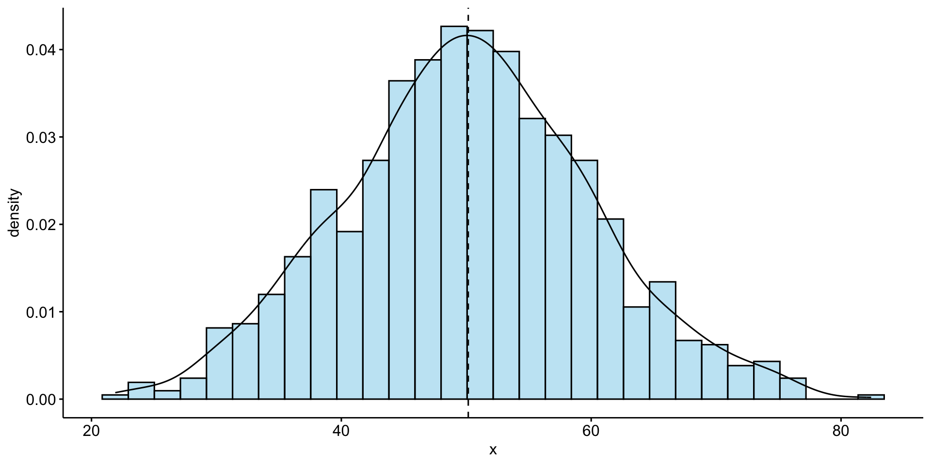
Univariate Analysis – Distribution of Bill Length

Univariate analysis focuses on a single variable at a time.

ggdensity(penguins, x = "bill_length_mm", add = "mean") +
  labs(title = "Distribution of Bill Length", x = "Bill Length (mm)")

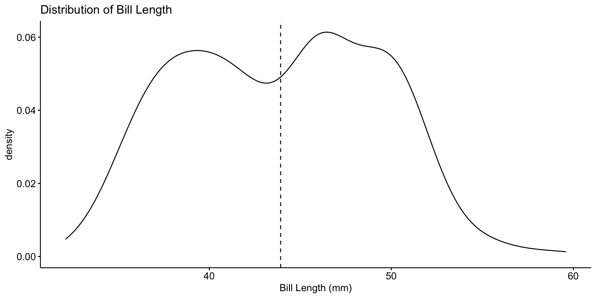
📌 Most bill lengths are between 35–55 mm. Some outliers exist.

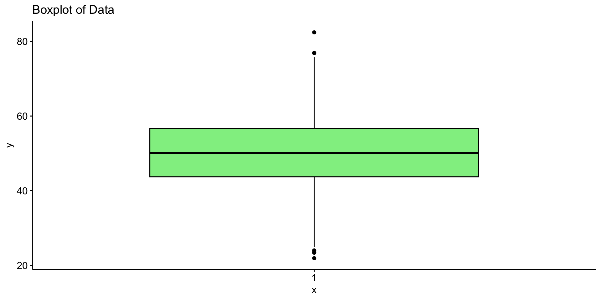
Boxplot for Outlier Detection

ggboxplot(penguins, x = "species", y = "bill_length_mm",
          color = "species", palette = "jco") +
  labs(title = "Bill Length Distribution by Species")

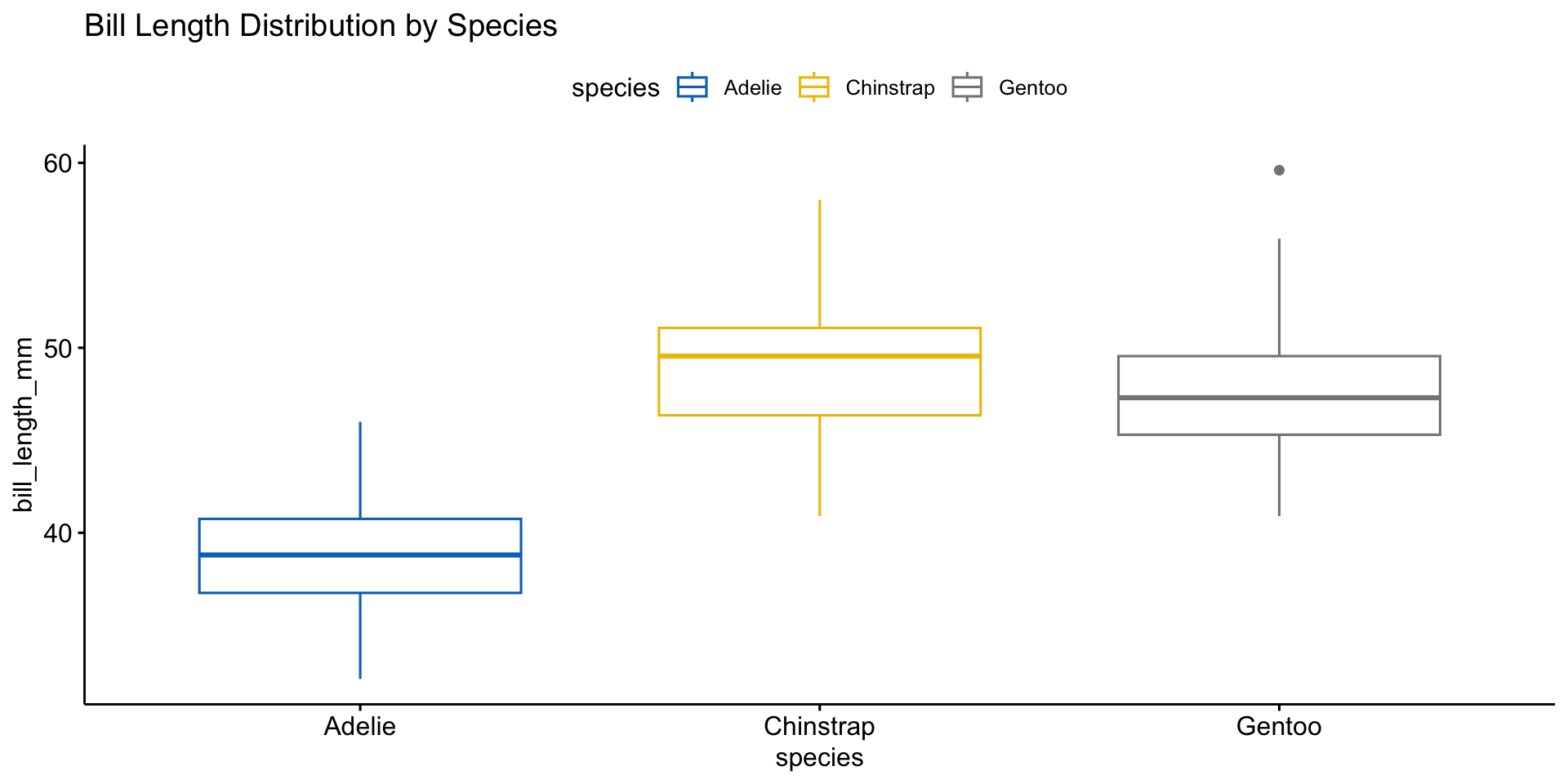
📌 Different species have distinct distributions. Outliers may need further investigation.

Bivariate Analysis

Variable Types	Plot Type
Categorical + Categorical	Bar plot (stacked or side-by-side)
Categorical + Continuous	Box plot; bar plot with summary stats
Continuous + Continuous	Scatter plot with regression line

ggscatter(penguins, x = "bill_length_mm", y = "bill_depth_mm",
          color = "species", add = "reg.line", conf.int = TRUE) +
  labs(title = "Bill Length vs. Bill Depth",
       x = "Bill Length (mm)", y = "Bill Depth (mm)")

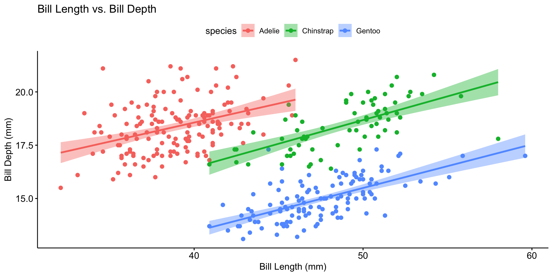
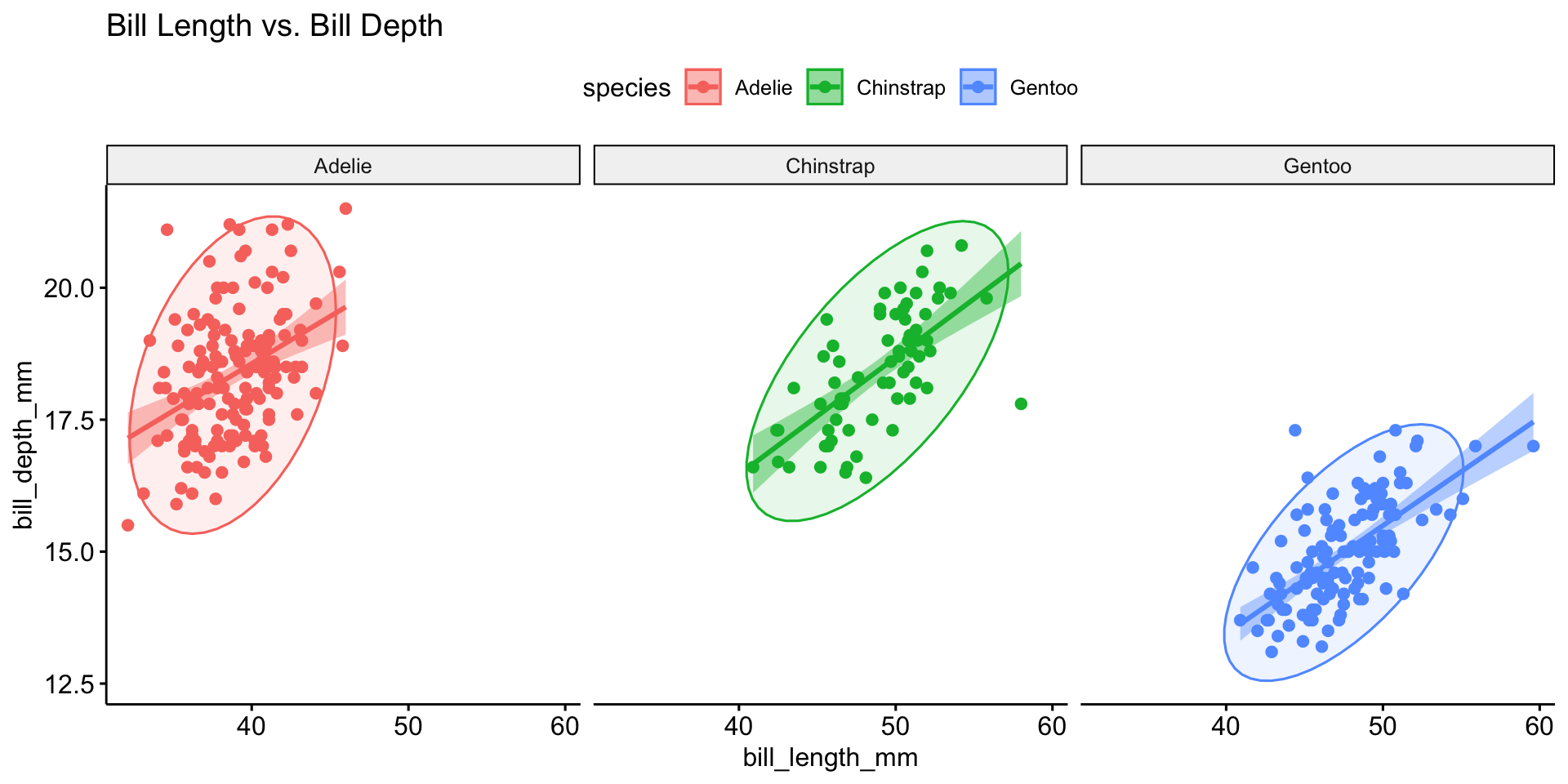
Multivariate Analysis

ggscatter(penguins, x = "bill_length_mm", y = "bill_depth_mm",
          color = "species", add = "reg.line", ellipse = TRUE, conf.int = TRUE) +
  labs(title = "Bill Length vs. Bill Depth") +
  facet_wrap(~species)

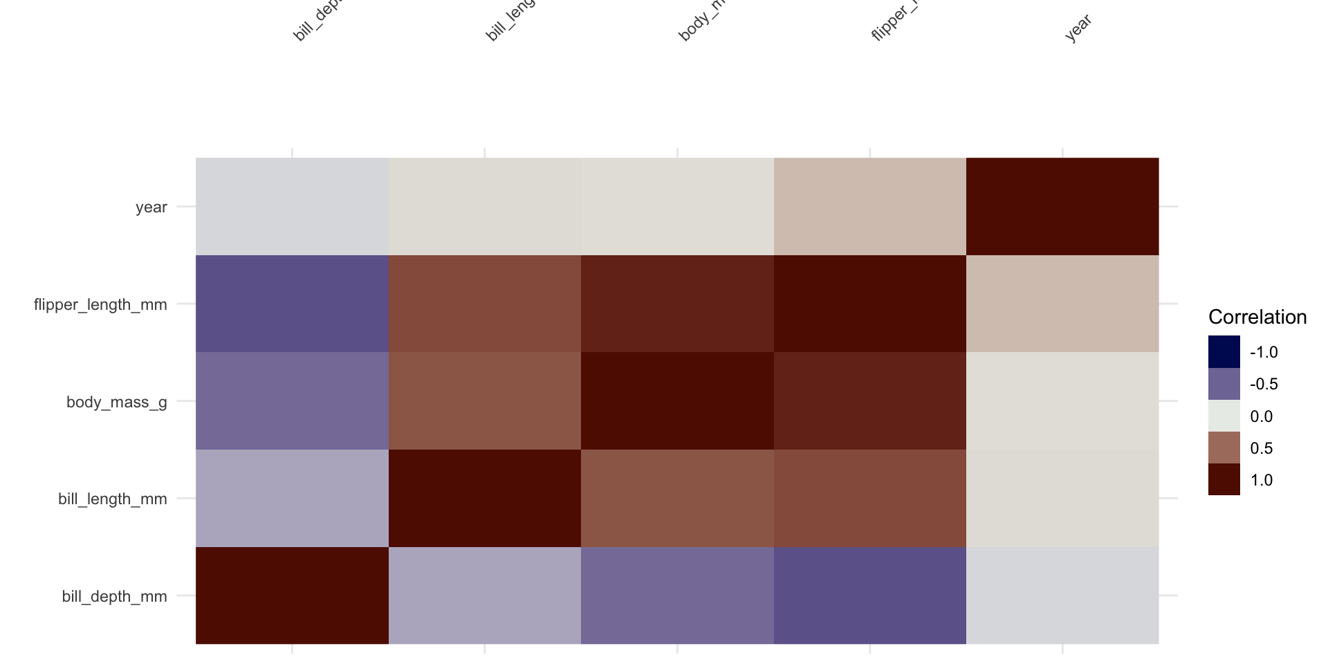
Correlation Analysis

• Correlation coefficients range from −1 to 1.
• Close to +1: strong positive relationship.
• Close to −1: strong negative relationship.
• Close to 0: no linear relationship.
• ⚠️ Correlation ≠ causation.

penguins |>
  select(where(is.numeric)) |>
  vis_cor()

Identify Data Issues

Duplicates:

df <- distinct(df)

Missing Data:

df <- drop_na(df)
# Or impute:
df <- mutate(df, x = if_else(is.na(x), mean(x, na.rm = TRUE), x))

Outlier Detection: IQR, Z-scores, or clustering-based methods.

Data Normality

Many statistical tests and models rely on the assumption that data is normally distributed.

What is the Central Limit Theorem?

• The CLT states that the sampling distribution of the sample mean approaches a normal distribution as sample size increases, regardless of the original distribution.
• This justifies using normal-based inference even when raw data isn’t normal.

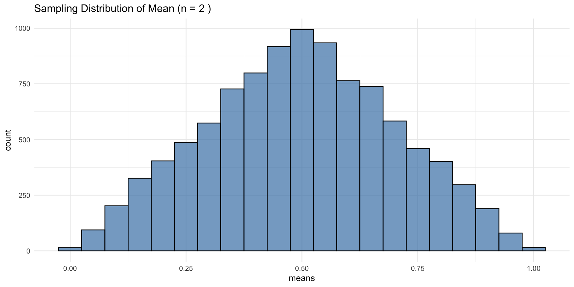
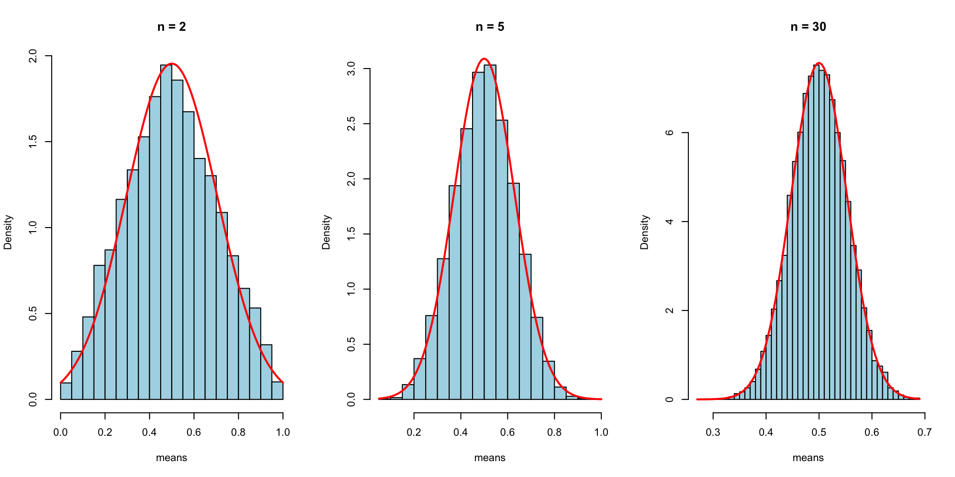
CLT in Action: Uniform Distribution

At n = 2, this may look normal, but the true distribution is triangular—CLT describes convergence, not instant normality

set.seed(123)
n    <- 2
sims <- 10000
means <- replicate(sims, mean(runif(n)))

ggplot(data.frame(means), aes(x = means)) +
  geom_histogram(binwidth = 0.05, fill = "steelblue", color = "black", alpha = 0.7) +
  ggtitle(paste("Sampling Distribution of Mean (n =", n, ")")) +
  theme_minimal()

CLT: Increasing Sample Size

As n increases, the distribution of sample means becomes normal even though the original data was uniform.

n_values <- c(2, 5, 30)
par(mfrow = c(1, 3))

for (n in n_values) {
  means <- replicate(sims, mean(runif(n)))
  hist(means, breaks = 30, main = paste("n =", n), col = "lightblue", probability = TRUE)
  curve(dnorm(x, mean = 0.5, sd = sqrt(1/12/n)), add = TRUE, col = "red", lwd = 2)
}

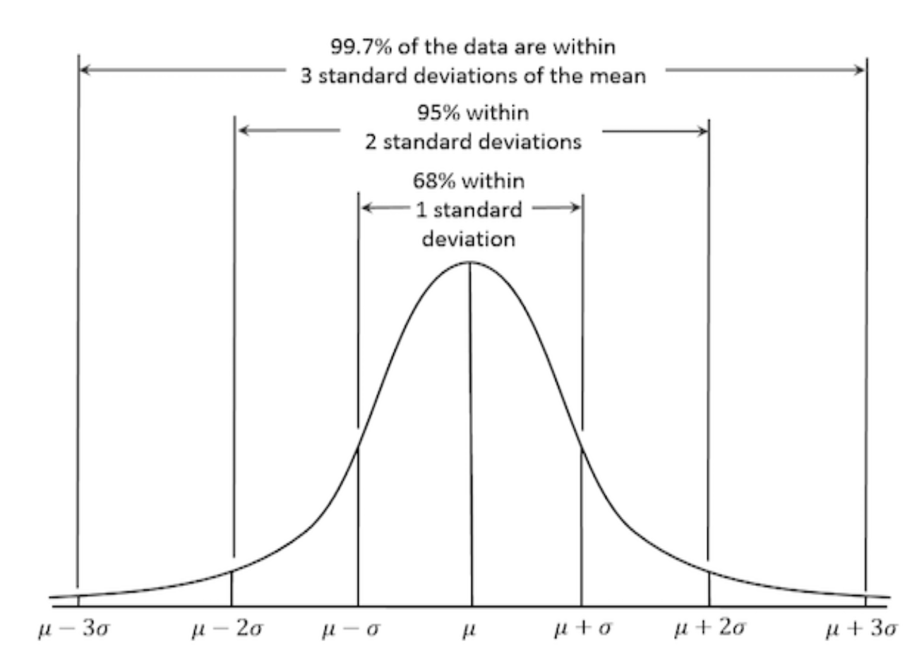
Properties of a Normal Distribution

• Symmetric about the mean
• Follows the empirical rule:
  • ~68% within 1 SD
  • ~95% within 2 SD
  • ~99.7% within 3 SD

set.seed(123)
data <- rnorm(1000, mean = 50, sd = 10)

Why Normality Matters

Many statistical techniques assume normality:

• t-tests / ANOVA — compare means between groups
• Linear regression (lm) — residuals should be normally distributed
• PCA — performs best with normally distributed features
• Confidence intervals — normality ensures accurate estimation

When data deviates from normality, these methods may produce inaccurate results.

Assessing Normality: Visual Methods

gghistogram(data, y = "density",
            bins = 30, fill = "skyblue",
            add = "mean", color = "black",
            add_density = TRUE)

ggboxplot(data, fill = "lightgreen",
          title = "Boxplot of Data")

Checking Normality with Q-Q Plots

• Points along the 45-degree line → normally distributed.
• Deviations suggest skewness or outliers.

ggqqplot(group_by(penguins, species), x = "body_mass_g", color = "species")

Statistical Tests for Normality

Test	Strengths	Weaknesses
Shapiro-Wilk	Sensitive; good for small samples	Too sensitive for large n
Kolmogorov-Smirnov	Works for any sample size	Less powerful for small n
Anderson-Darling	Emphasizes tails	Sensitive to sample size
Jarque-Bera	Tests skewness + kurtosis	Less reliable for small n

H₀ in all tests: data is normally distributed. Low p-value → reject H₀.

Normality Tests in R

shapiro.test(data)
#> 
#>  Shapiro-Wilk normality test
#> 
#> data:  data
#> W = 0.99838, p-value = 0.4765

ks.test(data, "pnorm", mean = mean(data), sd = sd(data))
#> 
#>  Asymptotic one-sample Kolmogorov-Smirnov test
#> 
#> data:  data
#> D = 0.014963, p-value = 0.9786
#> alternative hypothesis: two-sided

library(nortest)
ad.test(data)
#> 
#>  Anderson-Darling normality test
#> 
#> data:  data
#> A = 0.29653, p-value = 0.592

nest/map Pattern for Per-Group Testing

penguins |>
  drop_na() |>
  nest(data = -species) |>
  mutate(test          = map(data, ~shapiro.test(.x$body_mass_g)),
         glance_shapiro = map(test, broom::glance)) |>
  unnest(glance_shapiro)
#> # A tibble: 3 × 6
#>   species   data               test    statistic p.value method                 
#>   <fct>     <list>             <list>      <dbl>   <dbl> <chr>                  
#> 1 Adelie    <tibble [146 × 7]> <htest>     0.981  0.0423 Shapiro-Wilk normality…
#> 2 Gentoo    <tibble [119 × 7]> <htest>     0.986  0.261  Shapiro-Wilk normality…
#> 3 Chinstrap <tibble [68 × 7]>  <htest>     0.984  0.561  Shapiro-Wilk normality…

Dealing with Non-Normal Data

Option 1 — Transformations:

Transformation	When to Use
Log	Right-skewed, positive values
Square Root	Moderate right-skew, count data
Box-Cox	Unknown transformation needed
Yeo-Johnson	Like Box-Cox but works on negative values

log_data  <- log(data)
sqrt_data <- sqrt(data)

Option 2 — Nonparametric Methods

Use when data is not normally distributed:

# Wilcoxon (instead of t-test)
wilcox.test(Ozone ~ Month, data = airquality, subset = Month %in% c(5, 8))
#> 
#>  Wilcoxon rank sum test with continuity correction
#> 
#> data:  Ozone by Month
#> W = 127.5, p-value = 0.0001208
#> alternative hypothesis: true location shift is not equal to 0

# Kruskal-Wallis (instead of ANOVA)
kruskal.test(Ozone ~ Month, data = airquality)
#> 
#>  Kruskal-Wallis rank sum test
#> 
#> data:  Ozone by Month
#> Kruskal-Wallis chi-squared = 29.267, df = 4, p-value = 6.901e-06

# Spearman correlation (instead of Pearson)
cor.test(airquality$Ozone, airquality$Temp, method = "spearman")
#> 
#>  Spearman's rank correlation rho
#> 
#> data:  airquality$Ozone and airquality$Temp
#> S = 58778, p-value < 2.2e-16
#> alternative hypothesis: true rho is not equal to 0
#> sample estimates:
#>      rho 
#> 0.774043

Option 3 — Bootstrapping

Provides robust estimates without assuming normality:

library(boot)
boot_mean <- function(data, indices) mean(data[indices])
results <- boot(data, boot_mean, R = 1000)
plot(results)

Skewness

Skewness measures the asymmetry of a distribution:

• Positive skew: Longer right tail
• Negative skew: Longer left tail
• Symmetric: No skew (normal)

D’Agostino test for skewness:

moments::agostino.test(na.omit(penguins$body_mass_g))
#> 
#>  D'Agostino skewness test
#> 
#> data:  na.omit(penguins$body_mass_g)
#> skew = 0.46826, z = 3.44537, p-value = 0.0005703
#> alternative hypothesis: data have a skewness

On to modeling!

Now that the data is cleaned, understood, and modified, we can move on to modeling.

Data Budget

• In any modeling effort, it’s crucial to evaluate the performance of a model using different validation techniques to ensure a model can generalize to unseen data.

• But data is limited even in the age of “big data”.

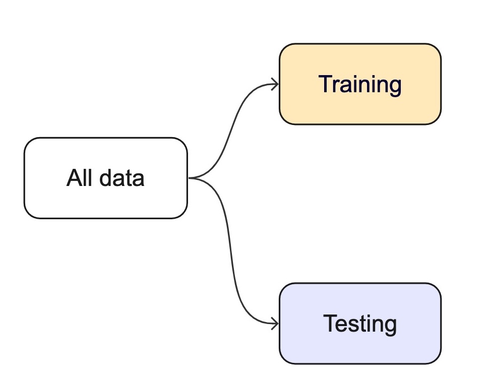
How we split data

• Splitting can be handled in many of ways. Typically, we base it off of a “hold out” percentage (e.g. 20%)

• These hold out cases are extracted randomly from the data set. (remember seeds?)

• The training set is usually the majority of the data and provides a sandbox for testing different modeling approaches.

• The test set is held in reserve until one or two models are chosen.

• The test set is then used as the final arbiter to determine the efficacy of the model.

Stratification

• In many cases, there is a structure to the data that would inhibit impartial splitting (e.g. a class, a region, a species, a sex, etc)

• Imagine you have a jar of M&Ms in different colors — red, blue, and green. You want to take some candies out to taste, but you want to make sure you get a fair mix of each color, not just grabbing a bunch of red ones by accident.

• Stratified resampling is like making sure that if your jar is 50% red, 30% blue, and 20% green, then the handful of candies you take keeps the same balance.

• In data science, we do the same thing when we pick samples from a dataset: we make sure that different groups (like categories of people, animals, or weather types) are still fairly represented!

Initial splits

• In tidymodels, the rsample package provides functions for creating initial splits of data.
• The initial_split() function is used to create a single split of the data.
• The prop argument defines the proportion of the data to be used for training.
• The default is 0.75, which means 75% of the data will be used for training and 25% for testing.

set.seed(101991)
(resample_split <- initial_split(penguins, prop = 0.8))
#> <Training/Testing/Total>
#> <275/69/344>

#Sanity check
69/344
#> [1] 0.2005814

Accessing the data:

• Once the data is split, we can access the training and testing data using the training() and testing() functions to extract the partitioned data from the full set:

penguins_train <- training(resample_split)
glimpse(penguins_train)
#> Rows: 275
#> Columns: 8
#> $ species           <fct> Gentoo, Adelie, Gentoo, Chinstrap, Gentoo, Chinstrap…
#> $ island            <fct> Biscoe, Torgersen, Biscoe, Dream, Biscoe, Dream, Dre…
#> $ bill_length_mm    <dbl> 46.2, 43.1, 46.2, 45.9, 46.5, 48.1, 45.2, 55.9, 38.1…
#> $ bill_depth_mm     <dbl> 14.9, 19.2, 14.4, 17.1, 13.5, 16.4, 17.8, 17.0, 17.0…
#> $ flipper_length_mm <int> 221, 197, 214, 190, 210, 199, 198, 228, 181, 195, 20…
#> $ body_mass_g       <int> 5300, 3500, 4650, 3575, 4550, 3325, 3950, 5600, 3175…
#> $ sex               <fct> male, male, NA, female, female, female, female, male…
#> $ year              <int> 2008, 2009, 2008, 2007, 2007, 2009, 2007, 2009, 2009…

penguins_test <- testing(resample_split)
glimpse(penguins_test)
#> Rows: 69
#> Columns: 8
#> $ species           <fct> Adelie, Adelie, Adelie, Adelie, Adelie, Adelie, Adel…
#> $ island            <fct> Torgersen, Torgersen, Torgersen, Biscoe, Biscoe, Bis…
#> $ bill_length_mm    <dbl> NA, 39.3, 36.6, 35.9, 38.8, 37.9, 39.2, 39.6, 36.7, …
#> $ bill_depth_mm     <dbl> NA, 20.6, 17.8, 19.2, 17.2, 18.6, 21.1, 17.2, 18.8, …
#> $ flipper_length_mm <int> NA, 190, 185, 189, 180, 172, 196, 196, 187, 205, 187…
#> $ body_mass_g       <int> NA, 3650, 3700, 3800, 3800, 3150, 4150, 3550, 3800, …
#> $ sex               <fct> NA, male, female, female, male, female, male, female…
#> $ year              <int> 2007, 2007, 2007, 2007, 2007, 2007, 2007, 2008, 2008…

Proportional Gaps — Before Stratification

Warning

Without stratification, random sampling can over- or under-represent groups. Compare the species proportions below — they don’t match.

# Dataset
(table(penguins$species) / nrow(penguins))
#> 
#>    Adelie Chinstrap    Gentoo 
#> 0.4418605 0.1976744 0.3604651
# Training Data
(table(penguins_train$species) / nrow(penguins_train))
#> 
#>    Adelie Chinstrap    Gentoo 
#> 0.4581818 0.1818182 0.3600000
# Testing Data
(table(penguins_test$species) / nrow(penguins_test))
#> 
#>    Adelie Chinstrap    Gentoo 
#> 0.3768116 0.2608696 0.3623188

Stratification Example

• A stratified random sample conducts a specified split within defined subsets of subsets, and then pools the results.

• Only one column can be used to define a strata, but grouping/mutate operations can be used to create a new column that can be used as a strata (e.g. species/island)

• In the case of the penguins data, we can stratify by species (think back to our nested/linear model approach)

• This ensures that the training and testing sets have the same proportion of each species as the original data.

# Set the seed
set.seed(123)

# Drop missing values and split the data
penguins <- drop_na(penguins)
penguins_strata <- initial_split(penguins, strata = species, prop = .8)

# Extract the training and testing sets

train_strata <- training(penguins_strata)
test_strata  <- testing(penguins_strata)

Proportional Alignment

# Check the proportions
# Dataset
table(penguins$species) / nrow(penguins)
#> 
#>    Adelie Chinstrap    Gentoo 
#> 0.4384384 0.2042042 0.3573574
# Training Data
table(train_strata$species) / nrow(train_strata)
#> 
#>    Adelie Chinstrap    Gentoo 
#> 0.4377358 0.2037736 0.3584906
# Testing Data
table(test_strata$species) / nrow(test_strata)
#> 
#>    Adelie Chinstrap    Gentoo 
#> 0.4411765 0.2058824 0.3529412

Modeling

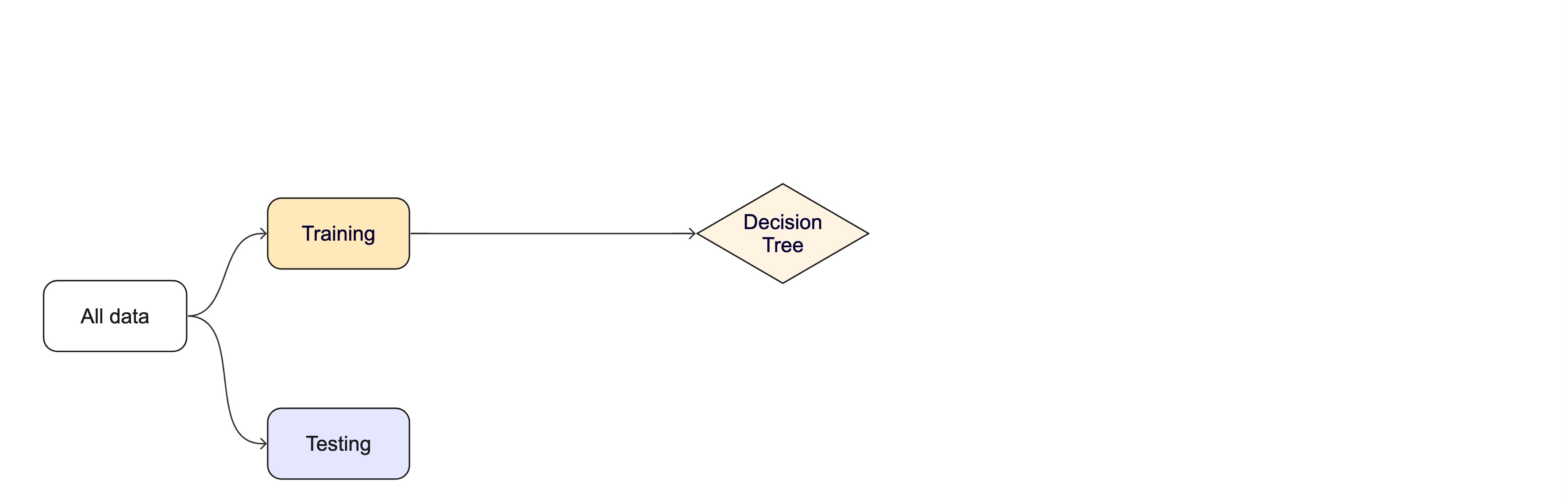
• Once the data is split, we can decide what type of model to invoke.

• Often, users simply pick a well known model type or class for a type of problem (Classic Conceptual Model)

• We will learn more about model types and uses next week!

• For now, just know that the training data is used to fit a model.

• If we are certain about the model, we can use the test data to evaluate the model.

Modeling Options

• But, there are many types of models, with different assumptions, behaviors, and qualities, that make some more applicable to a given dataset!

• Most models have some type of parameterization, that can often be tuned.

• Testing combinations of model and tuning parameters also requires some combination of training/testing splits.

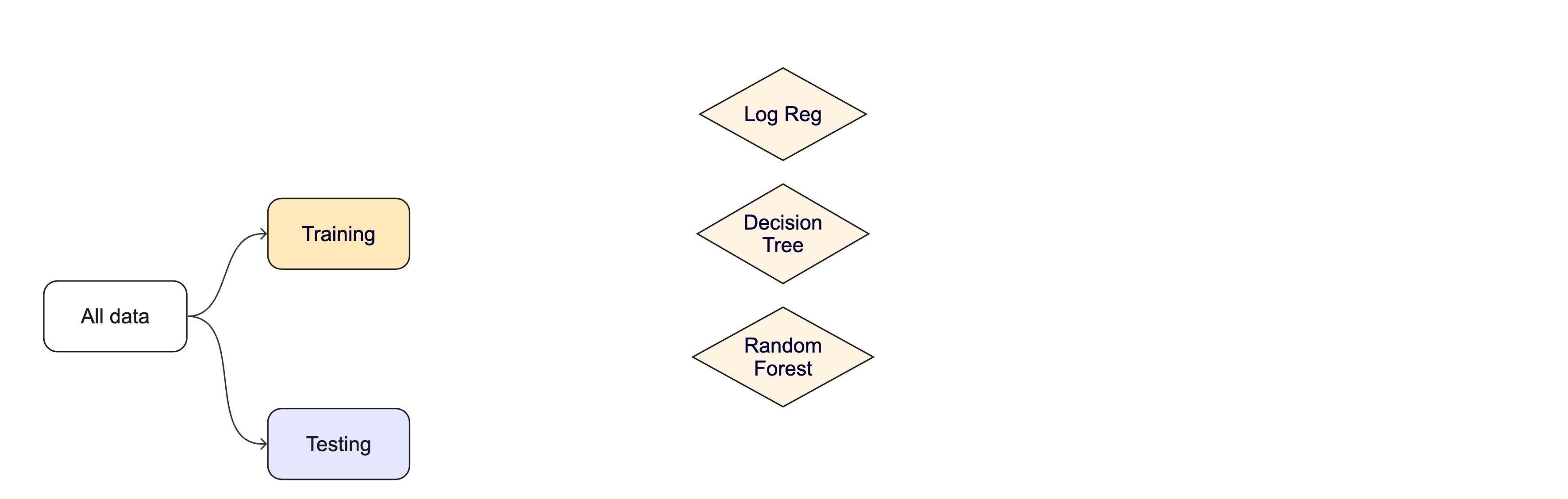
Modeling Options

What if we want to compare more models?

And/or more model configurations?

And we want to understand if these are important differences?

How can we use the training data to compare and evaluate different models? 🤔

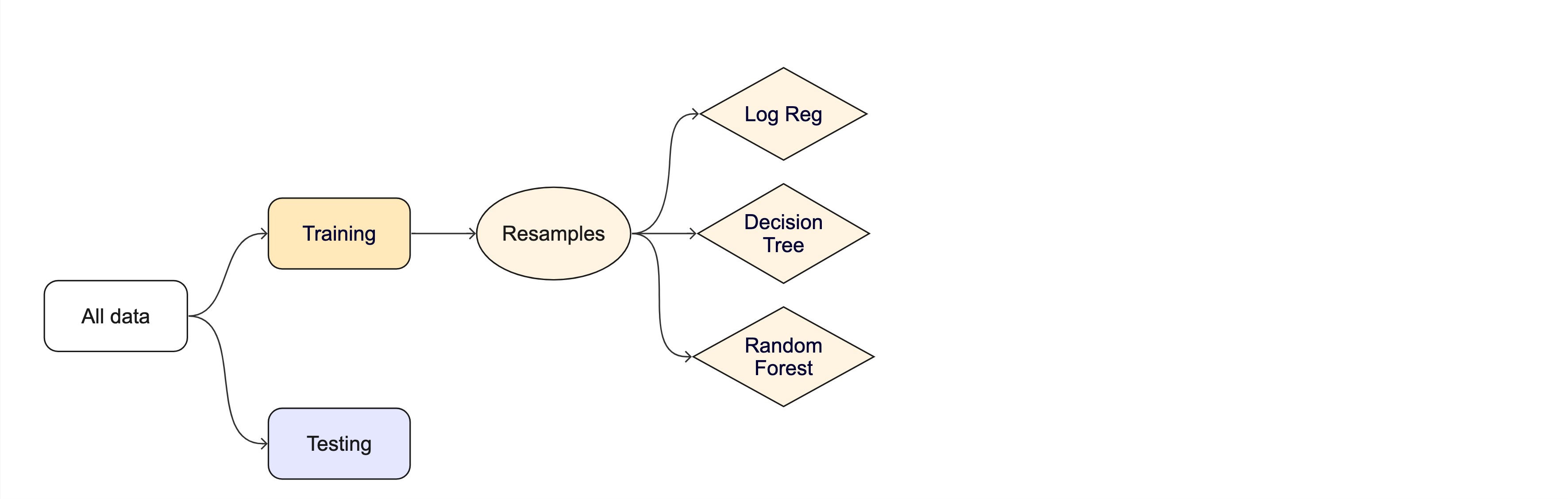
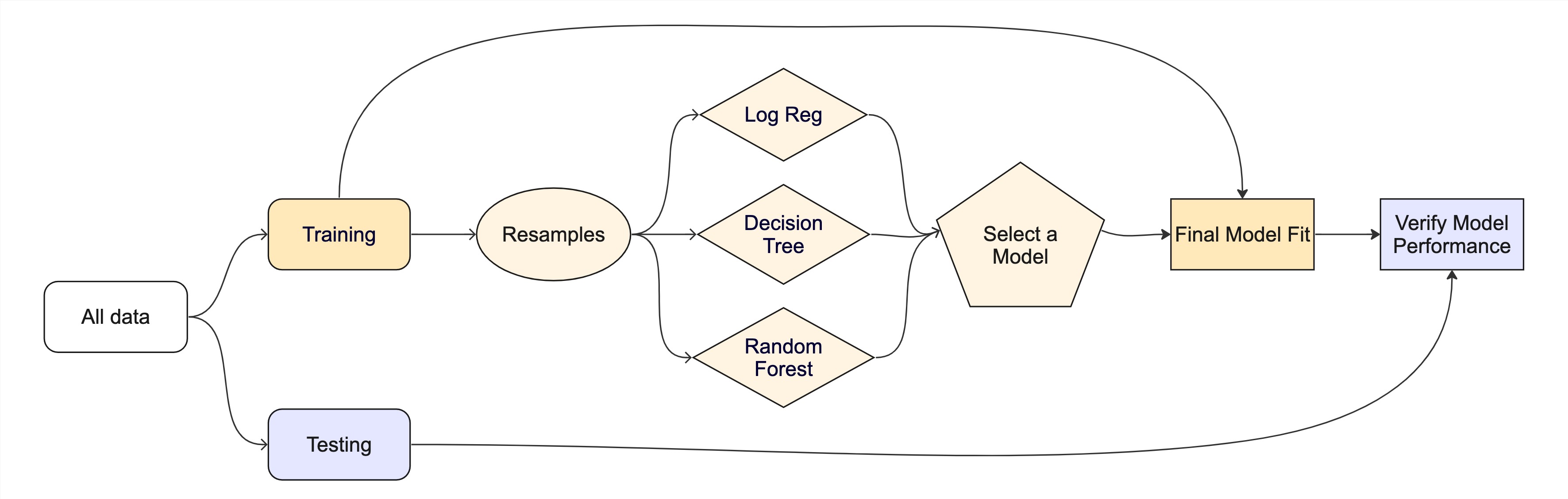
Resampling

• Testing combinations of model and tuning parameters also requires some combination of training/testing splits.

• Resampling methods, such as cross-validation and bootstrapping, are empirical simulation systems that help facilitate this.

• They create a series of data sets similar to the initial training/testing split.

• In the first level of the diagram to the right, we first split the original data into training/testing sets. Then, the training set is chosen for resampling.

Key Resampling Methods

Warning

Resampling is always used with the training set.

Resampling is a key step in model validation and assessment. The rsample package provides tools to create resampling strategies such as cross-validation, bootstrapping, and validation splits.

1. K-Fold Cross-Validation: The dataset is split into multiple “folds” (e.g., 5-fold or 10-fold), where each fold is used as a validation set while the remaining data is used for training.

   Example (10-fold): On iteration 1, folds 2–10 become the training set and fold 1 is held out for assessment. On iteration 2, fold 2 is held out and folds 1, 3–10 are trained on. After 10 iterations every row has been predicted exactly once from a model it did not train on — and we average the 10 metric values to get a more stable estimate of skill.

2. Bootstrap Resampling: Samples are drawn with replacement from the training dataset to generate multiple datasets, which are used to train and test the model.

3. Monte Carlo Resampling (Repeated Train-Test Splits): Randomly splits data multiple times.

4. Validation Split: Creates a single training and testing partition.

Cross-validation

Cross-validation

Cross-validation

penguins_train |> glimpse() 
#> Rows: 275
#> Columns: 8
#> $ species           <fct> Gentoo, Adelie, Gentoo, Chinstrap, Gentoo, Chinstrap…
#> $ island            <fct> Biscoe, Torgersen, Biscoe, Dream, Biscoe, Dream, Dre…
#> $ bill_length_mm    <dbl> 46.2, 43.1, 46.2, 45.9, 46.5, 48.1, 45.2, 55.9, 38.1…
#> $ bill_depth_mm     <dbl> 14.9, 19.2, 14.4, 17.1, 13.5, 16.4, 17.8, 17.0, 17.0…
#> $ flipper_length_mm <int> 221, 197, 214, 190, 210, 199, 198, 228, 181, 195, 20…
#> $ body_mass_g       <int> 5300, 3500, 4650, 3575, 4550, 3325, 3950, 5600, 3175…
#> $ sex               <fct> male, male, NA, female, female, female, female, male…
#> $ year              <int> 2008, 2009, 2008, 2007, 2007, 2009, 2007, 2009, 2009…

nrow(penguins_train) * 1/10
#> [1] 27.5

vfold_cv(penguins_train, v = 10) # v = 10 is default
#> #  10-fold cross-validation 
#> # A tibble: 10 × 2
#>    splits           id    
#>    <list>           <chr> 
#>  1 <split [247/28]> Fold01
#>  2 <split [247/28]> Fold02
#>  3 <split [247/28]> Fold03
#>  4 <split [247/28]> Fold04
#>  5 <split [247/28]> Fold05
#>  6 <split [248/27]> Fold06
#>  7 <split [248/27]> Fold07
#>  8 <split [248/27]> Fold08
#>  9 <split [248/27]> Fold09
#> 10 <split [248/27]> Fold10

Cross-validation

What is in this?

penguins_folds <- vfold_cv(penguins_train)
penguins_folds$splits[1:3]
#> [[1]]
#> <Analysis/Assess/Total>
#> <247/28/275>
#> 
#> [[2]]
#> <Analysis/Assess/Total>
#> <247/28/275>
#> 
#> [[3]]
#> <Analysis/Assess/Total>
#> <247/28/275>

Note

Here is another example of a list column enabling the storage of non-atomic types in tibble

Important

Set the seed when creating resamples

Alternate resampling schemes

Bootstrapping

Bootstrapping

set.seed(3214)
bootstraps(penguins_train)
#> # Bootstrap sampling 
#> # A tibble: 25 × 2
#>    splits            id         
#>    <list>            <chr>      
#>  1 <split [275/96]>  Bootstrap01
#>  2 <split [275/105]> Bootstrap02
#>  3 <split [275/108]> Bootstrap03
#>  4 <split [275/111]> Bootstrap04
#>  5 <split [275/102]> Bootstrap05
#>  6 <split [275/98]>  Bootstrap06
#>  7 <split [275/92]>  Bootstrap07
#>  8 <split [275/97]>  Bootstrap08
#>  9 <split [275/100]> Bootstrap09
#> 10 <split [275/99]>  Bootstrap10
#> # ℹ 15 more rows

Monte Carlo Cross-Validation

set.seed(322)
mc_cv(penguins_train, times = 10)
#> # Monte Carlo cross-validation (0.75/0.25) with 10 resamples 
#> # A tibble: 10 × 2
#>    splits           id        
#>    <list>           <chr>     
#>  1 <split [206/69]> Resample01
#>  2 <split [206/69]> Resample02
#>  3 <split [206/69]> Resample03
#>  4 <split [206/69]> Resample04
#>  5 <split [206/69]> Resample05
#>  6 <split [206/69]> Resample06
#>  7 <split [206/69]> Resample07
#>  8 <split [206/69]> Resample08
#>  9 <split [206/69]> Resample09
#> 10 <split [206/69]> Resample10

Validation set

set.seed(853)
penguins_val_split <- initial_validation_split(penguins)
penguins_val_split
#> <Training/Validation/Testing/Total>
#> <199/67/67/333>
validation_set(penguins_val_split)
#> # A tibble: 1 × 2
#>   splits           id        
#>   <list>           <chr>     
#> 1 <split [199/67]> validation

A validation set is just another type of resample

The whole game - status update

Unit Example

Can we predict if a plot of land is forested?

• Interested in classification models
• We have a dataset of 7,107 6000-acre hexagons in Washington state
• Each hexagon has a nominal outcome, forested, with levels "Yes" and "No"

Data on forests in Washington

• The U.S. Forest Service maintains ML models to predict whether a plot of land is “forested.”
• This classification is important for all sorts of research, legislation, and land management purposes.
• Plots are typically remeasured every 10 years and this dataset contains the most recent measurement per plot.
• Type ?forested to learn more about this dataset, including references.

Data on forests in Washington

library(tidymodels)
library(forested)
dim(forested)
#> [1] 7107   19

• One observation from each of 7,107 6000-acre hexagons in Washington state.

• A nominal outcome, forested, with levels "Yes" and "No", measured on-the-ground (expensive, slow).

table(forested$forested)
#> 
#>  Yes   No 
#> 3894 3213

• 18 remotely-sensed and easily-accessible predictors (cheap, fast, wall-to-wall coverage).

• The ML framing: use cheap, abundant predictors to estimate an expensive ground-truth label so the Forest Service can predict forest cover without sending a crew to every hexagon.

names(forested)
#>  [1] "forested"         "year"             "elevation"        "eastness"        
#>  [5] "northness"        "roughness"        "tree_no_tree"     "dew_temp"        
#>  [9] "precip_annual"    "temp_annual_mean" "temp_annual_min"  "temp_annual_max" 
#> [13] "temp_january_min" "vapor_min"        "vapor_max"        "canopy_cover"    
#> [17] "lon"              "lat"              "land_type"

Data splitting and spending

The initial split

set.seed(123)
forested_split <- initial_split(forested, prop = .8, strata = tree_no_tree)
forested_split
#> <Training/Testing/Total>
#> <5685/1422/7107>

Accessing the data

forested_train <- training(forested_split)
forested_test  <- testing(forested_split)

nrow(forested_train)
#> [1] 5685
nrow(forested_test)
#> [1] 1422

K-Fold Cross-Validation

# Load the dataset
set.seed(123)

# Create a 10-fold cross-validation object
(forested_folds <- vfold_cv(forested_train, v = 10))
#> #  10-fold cross-validation 
#> # A tibble: 10 × 2
#>    splits             id    
#>    <list>             <chr> 
#>  1 <split [5116/569]> Fold01
#>  2 <split [5116/569]> Fold02
#>  3 <split [5116/569]> Fold03
#>  4 <split [5116/569]> Fold04
#>  5 <split [5116/569]> Fold05
#>  6 <split [5117/568]> Fold06
#>  7 <split [5117/568]> Fold07
#>  8 <split [5117/568]> Fold08
#>  9 <split [5117/568]> Fold09
#> 10 <split [5117/568]> Fold10

How do you fit a model in R?

• lm for linear model <– The one we have looked at!

• glmnet for regularized regression

• keras for regression using TensorFlow

• stan for Bayesian regression using Stan

• spark for large data sets using spark

• brulee for regression using torch (PyTorch)

Challenge

• All of these models have different syntax and functions
• How do you keep track of all of them?
• How do you know which one to use?
• How would you compare them?

Comparing 3-5 of these models is a lot of work using functions for diverse packages.

The tidymodels advantage

• In the tidymodels framework, all models are created using the same syntax:
  • This makes it easy to compare models
  • This makes it easy to switch between models
  • This makes it easy to use the same model with different engines (packages)
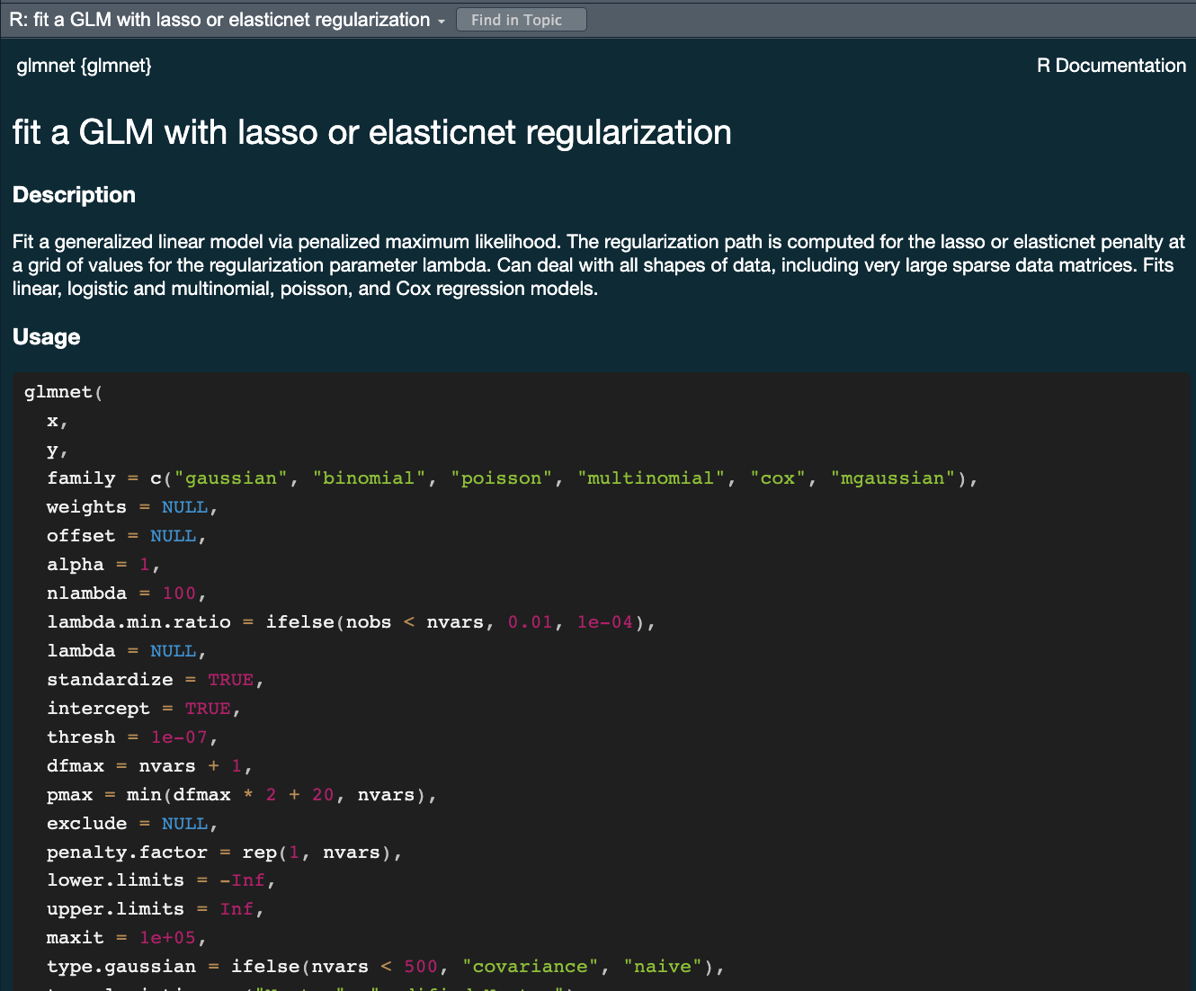
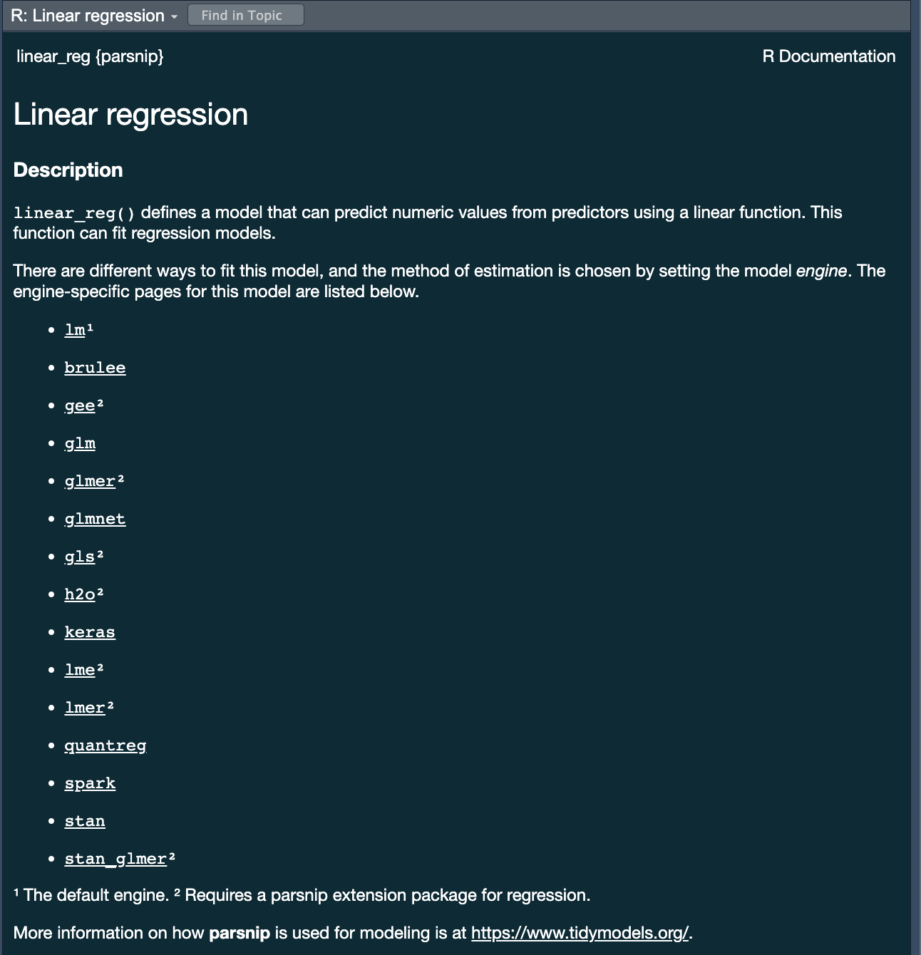
• The parsnip package provides a consistent interface to many models
• For example, to fit a linear model you would be able to access the linear_reg() function

?linear_reg

A tidymodels prediction will …

• always be inside a tibble
• have column names and types that are unsurprising and predictable
• ensure the number of rows in new_data and the output are the same

To specify a model

• Choose a model
• Specify an engine
• Set the mode

Specify a model: Type

Next week we will discuss model types more thoroughly. For now, we will focus on two types:

1. Logistic Regression

logistic_reg()
#> Logistic Regression Model Specification (classification)
#> 
#> Computational engine: glm

decision_tree()
#> Decision Tree Model Specification (unknown mode)
#> 
#> Computational engine: rpart

We chose these two because they are robust, simple models that fit our goal of predicting a binary condition/class (forested/not forested)

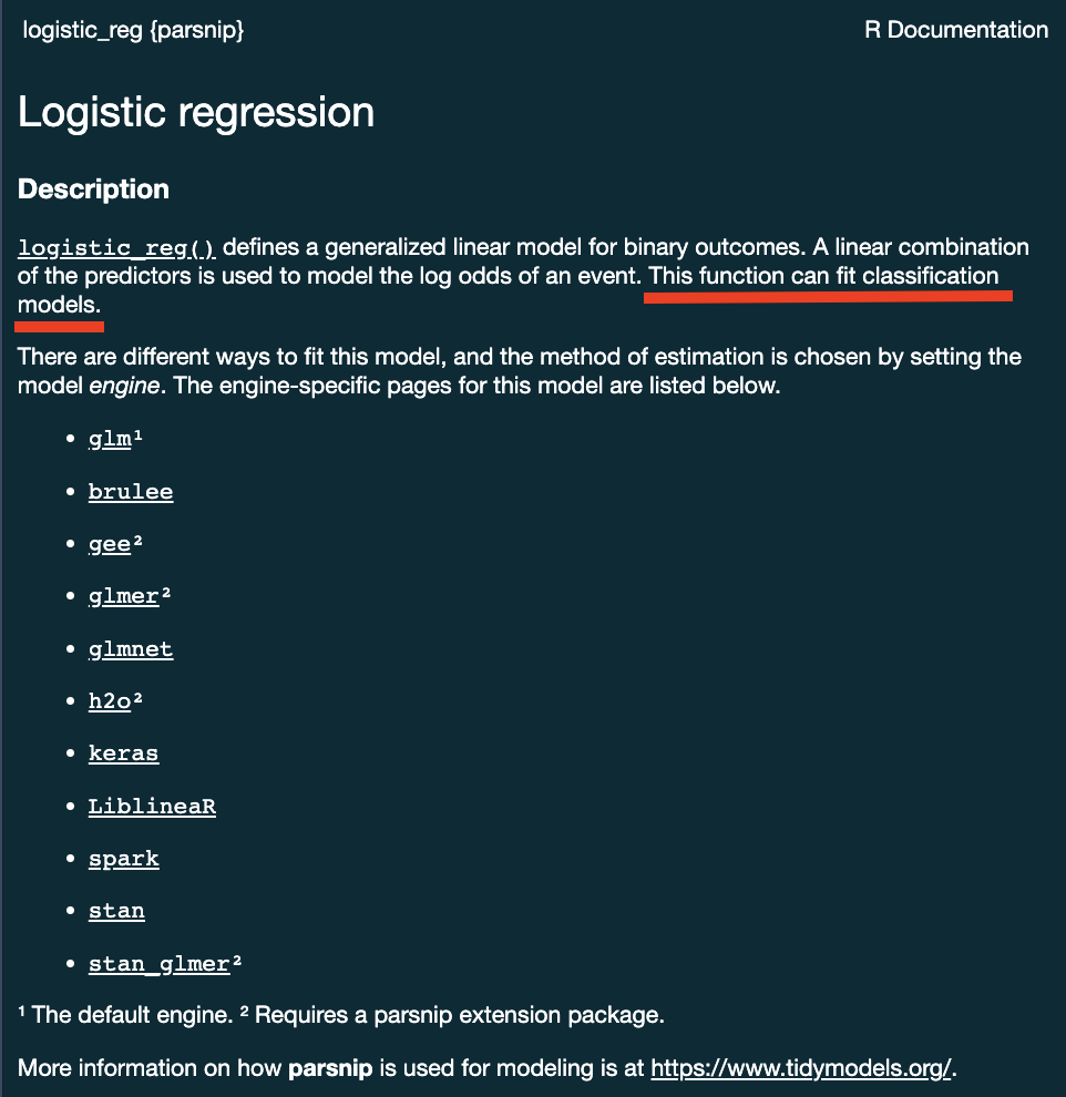
Specify a model: engine

• Choose a model
• Specify an engine
• Set the mode

?logistic_reg()

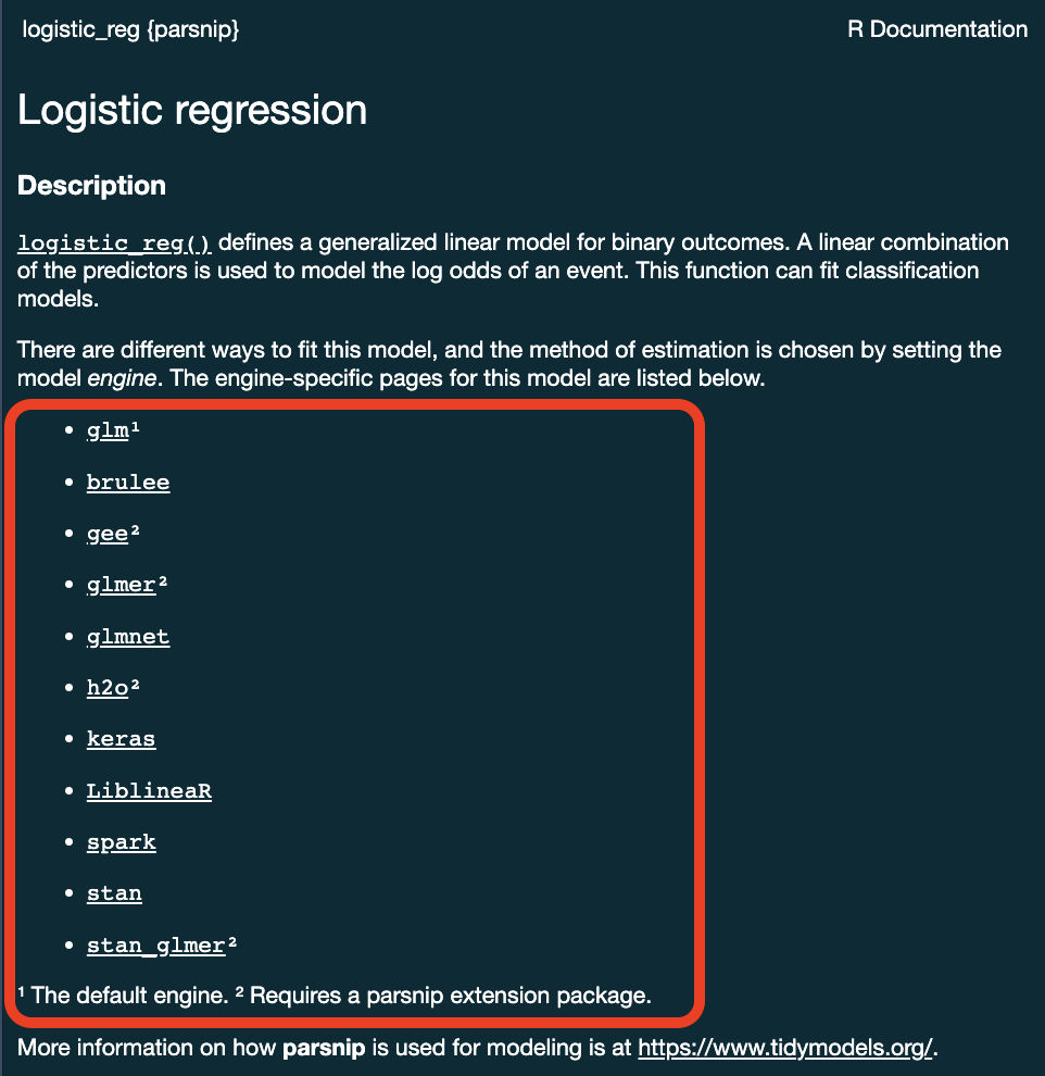
Specify a model: engine

logistic_reg() %>%
  set_engine("glmnet")
#> Logistic Regression Model Specification (classification)
#> 
#> Computational engine: glmnet

logistic_reg() %>%
  set_engine("stan")
#> Logistic Regression Model Specification (classification)
#> 
#> Computational engine: stan

Specify a model: mode

• Choose a model
• Specify an engine
• Set the mode

?logistic_reg()

Specify a model: mode

Some models have a limited set of modes …

logistic_reg()
#> Logistic Regression Model Specification (classification)
#> 
#> Computational engine: glm

. . .

Others require specification …

decision_tree()
#> Decision Tree Model Specification (unknown mode)
#> 
#> Computational engine: rpart

decision_tree() %>% 
  set_mode("classification")
#> Decision Tree Model Specification (classification)
#> 
#> Computational engine: rpart

All available models are listed at https://www.tidymodels.org/find/parsnip/

To specify a model

• Choose a model
• Specify an engine
• Set the mode

Two algorithms to try

We have a problem (predict whether a hexagon is forested), data (forested_train), and a way to evaluate predictions. Before we wire up the full tidymodels plumbing, let’s look at the two models we’ll compare today.

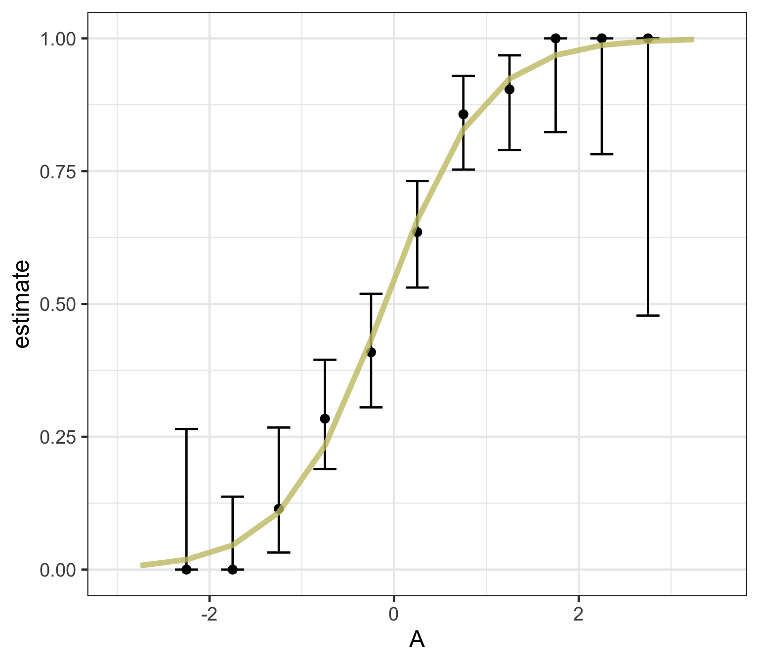
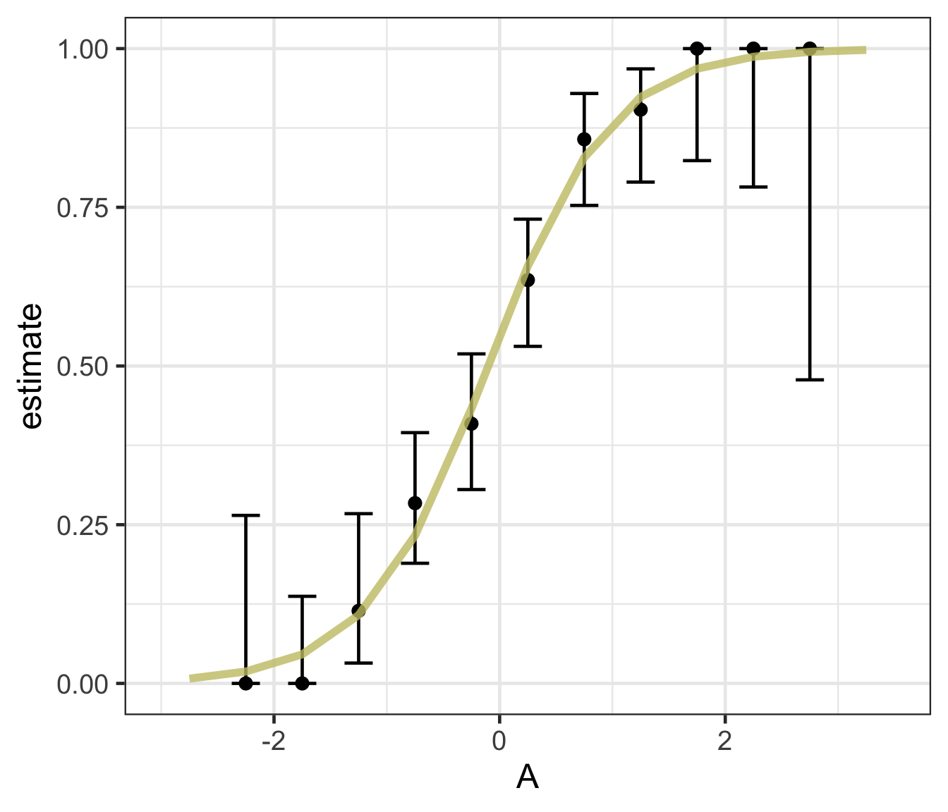
Logistic regression

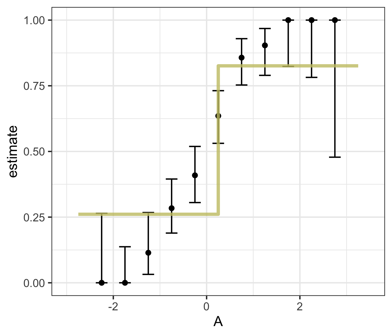
• Logistic regression predicts probability—instead of a straight line, it gives an S-shaped curve that estimates how likely an outcome (e.g., is forested) is based on a predictor (e.g., rainfall and temperature).

• The dots in the plot show the actual proportion of “successes” (e.g., is forested) within different bins of the predictor variable(s) (A).

• The vertical error bars represent uncertainty—showing a range where the true probability might fall.

• Logistic regression helps answer “how likely” questions—e.g., “How likely is someone to pass based on their study hours?” rather than just predicting a yes/no outcome.

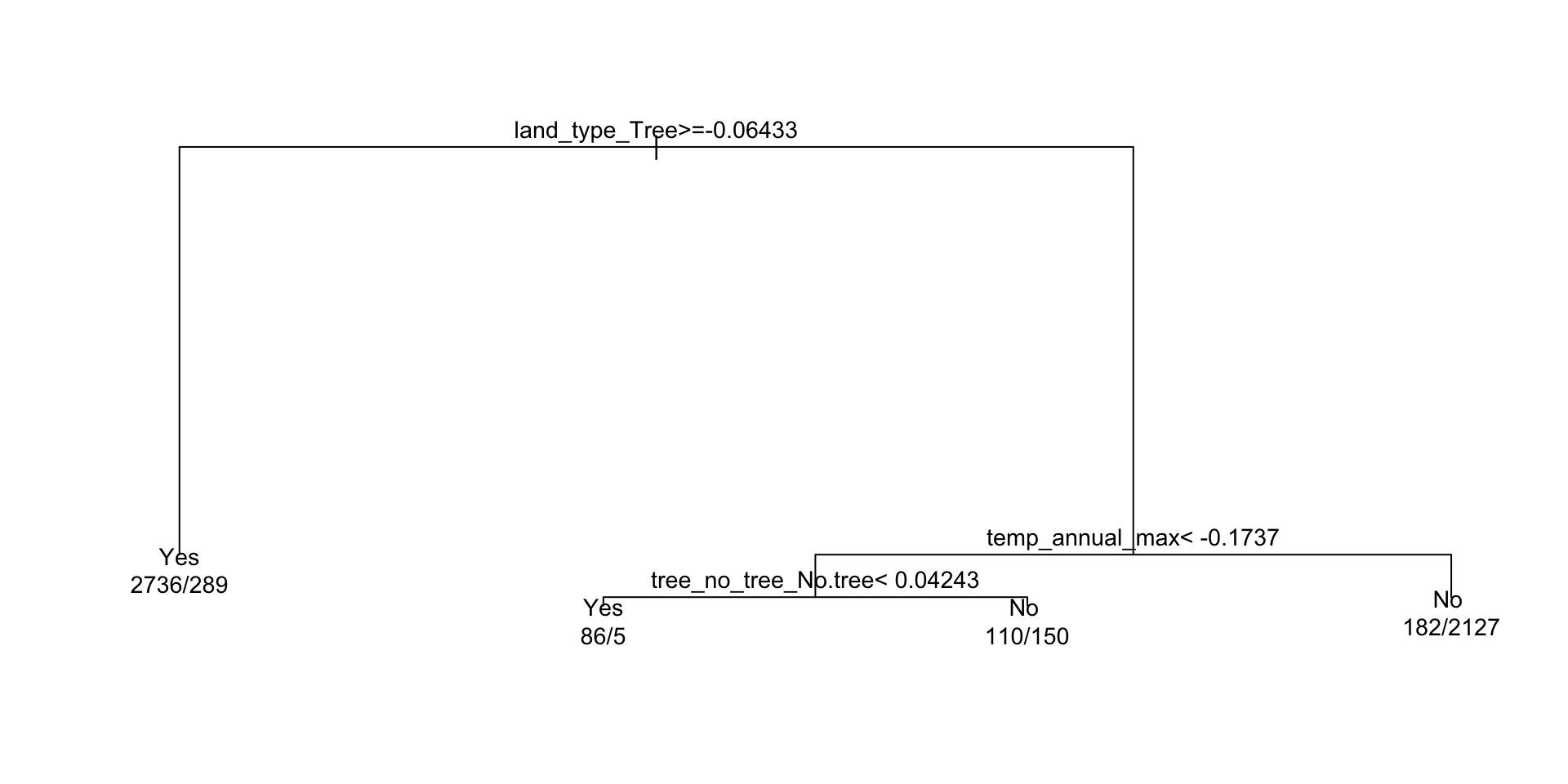
Decision trees — structure & pruning

• Series of splits or if/then statements based on predictors

• First the tree grows until some condition is met (maximum depth, no more data)

• Then the tree is pruned to reduce its complexity

• Each terminal leaf predicts a class (or, for regression, a numeric value)

Decision trees — what predictions look like

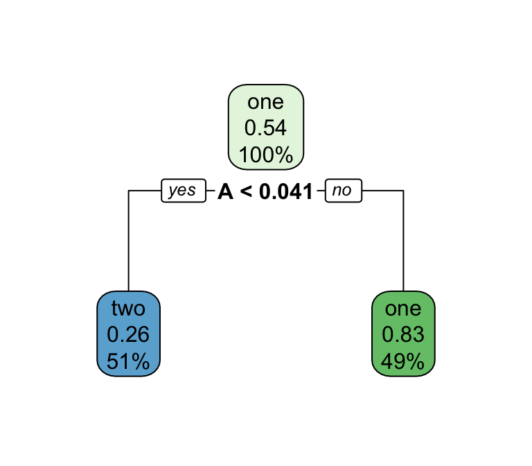
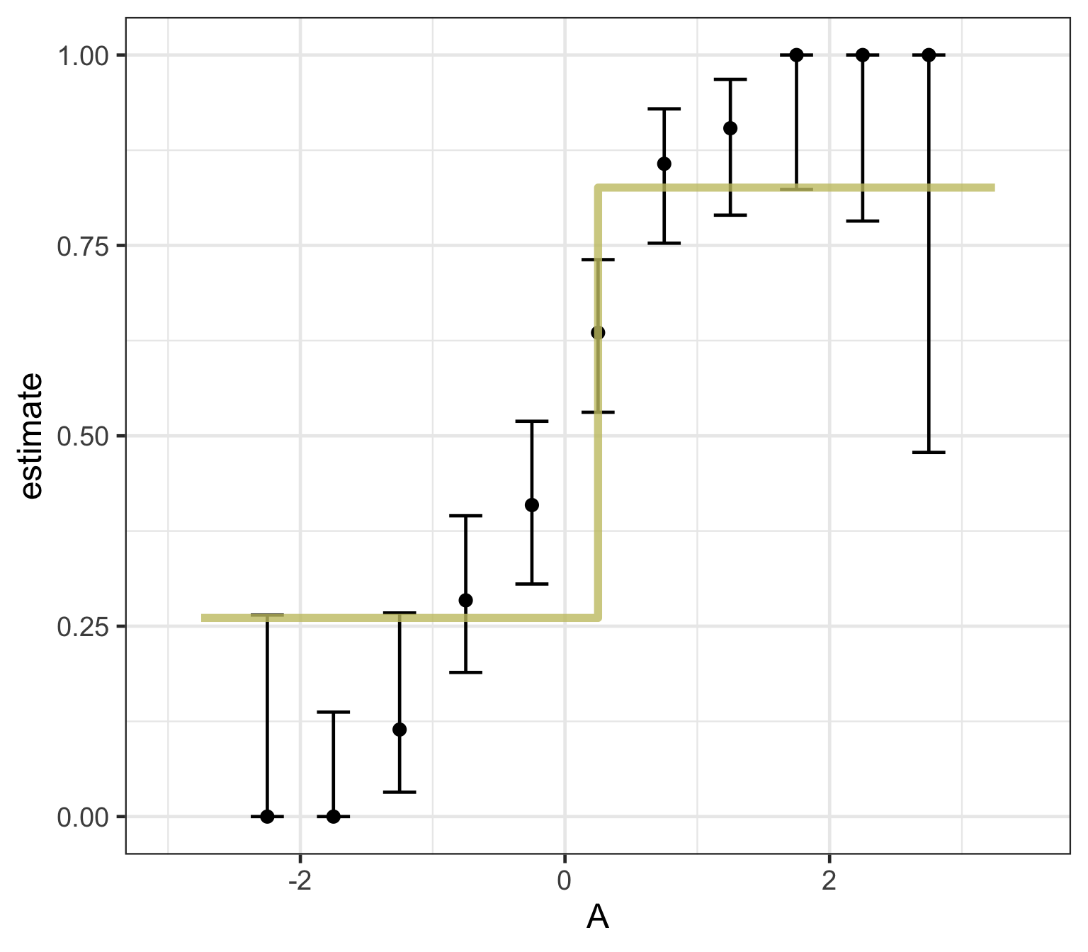
A tree’s decision boundary is stepwise — in contrast to the smooth S-curve of logistic regression.

When would you reach for each?

Logistic regression

• Smooth, monotonic decision boundary
• Returns calibrated probabilities, not just a class
• Coefficients are interpretable (log-odds per predictor)
• Sensitive to predictor scale → benefits from normalization
• Assumes a (largely) linear relationship on the log-odds scale

Decision trees

• Step-wise, rectangular splits on predictors
• Handles non-linearities and interactions natively
• No need to scale, dummy-encode, or worry about collinearity
• Easy to explain visually, but a single tree can overfit and is unstable across samples
• Sets up ensemble methods (random forest, boosting) next week

What algorithm is best for estimating forested plots?

We can only really know by testing them … but we know the options!

Logistic regression

Decision trees

Feature engineering with recipes

Why preprocess?

• A raw formula (forested ~ .) would send features to the model untouched.

• But many models care how their features look — different scales, skewed distributions, missing values, or categorical levels can bias the fit.

• recipes lets us declare a preprocessing pipeline once, estimate its parameters from the training data, and apply it consistently to every new data set (folds, test set, future predictions).

Important

Preprocessing parameters (means, sds, imputed values, PCA loadings) are learned only on the training set — this prevents data leakage from test data into the fit.

Data Normalization in tidymodels

• We’ve now seen why distributions matter and how to detect non-normality.
• In the recipes framework, normalization is declared once and applied consistently to every split — preventing data leakage.
• The same step_*() functions handle min-max scaling, z-score standardization, power transforms, and more.

Common Normalization Techniques

Technique	Idea	When to use	step_*
Min-max	rescale to \([0, 1]\): \(x' = \frac{x - x_\text{min}}{x_\text{max} - x_\text{min}}\)	Need a bounded range; beware outliers	step_range()
Z-score	center + scale: \(x' = \frac{x - \mu}{\sigma}\)	Symmetric-ish features, different units	step_normalize()
Power	Box-Cox (positive) or Yeo-Johnson (any sign) estimate an optimal power transform	Reshape skew toward normality before scaling	step_YeoJohnson(), step_BoxCox()
Log	\(x' = \log(x)\)	Right-skewed positive data (e.g. streamflow)	step_log()
PCA	project to a lower-dimensional basis that preserves variance	Many correlated numeric predictors	step_pca()

Tip

For environmental variables (streamflow, precipitation, concentrations) log is by far the most common first move — they’re almost always right-skewed.

Other Feature Engineering Tasks

Beyond scaling, three recipes moves you’ll reach for most often in water resources:

Handling missing values

• step_impute_mean() / step_impute_median() — fast, parametric fill
• step_impute_knn() — use neighboring rows (preserves covariance structure)

Encoding categorical variables

• step_dummy(all_nominal_predictors()) — one-hot encodes factors
• step_other() — collapses rare levels into “other”

Creating interaction terms

• step_interact(terms = ~ aridity:p_mean) — add variable products when the effect of one predictor depends on another

Note

The full step_* catalog (text, splines, binning, dimension reduction, …) lives at https://recipes.tidymodels.org/reference/. Search there when you need something not listed here.

Implementing a recipe in tidymodels

1. Declare a recipe() with a formula + training data.

2. Add step_*() preprocessing operations (imputation, dummies, normalization, …).

3. prep() estimates the transformation parameters from the training data.

4. bake() applies those transformations to any data set (training, test, new).

Example Workflow

library(tidymodels)

(recipe_obj <- recipe(flipper_length_mm ~
                       bill_length_mm + body_mass_g +
                       sex + island + species,
                      data = penguins) |>
  step_impute_mean(all_numeric_predictors()) |>
  step_dummy(all_factor_predictors()) |>
  step_normalize(all_numeric_predictors()))

# Prepare and apply transformations
prep_recipe     <- prep(recipe_obj, training = penguins)

normalized_data <- bake(prep_recipe, new_data = NULL) |>
  mutate(species = penguins$species) |>
  drop_na()

head(normalized_data)
#> # A tibble: 6 × 9
#>   bill_length_mm body_mass_g flipper_length_mm sex_male island_Dream
#>            <dbl>       <dbl>             <int>    <dbl>        <dbl>
#> 1         -0.895      -0.568               181    0.990       -0.764
#> 2         -0.822      -0.506               186   -1.01        -0.764
#> 3         -0.675      -1.19                195   -1.01        -0.764
#> 4         -1.33       -0.940               193   -1.01        -0.764
#> 5         -0.858      -0.692               190    0.990       -0.764
#> 6         -0.931      -0.723               181   -1.01        -0.764
#> # ℹ 4 more variables: island_Torgersen <dbl>, species_Chinstrap <dbl>,
#> #   species_Gentoo <dbl>, species <fct>

Explanation:

• recipe() defines preprocessing steps for modeling.

• step_impute_mean(all_numeric_predictors()) fills missing numeric values with the column mean (estimated on training data).

• step_dummy(all_factor_predictors()) creates dummy variables for categorical predictors.

• step_normalize(all_numeric_predictors()) standardizes all numerical predictors (mean 0, sd 1).

• prep() estimates parameters for transformations.

• bake() applies the transformations to the dataset.

A recipe for our running example

Back to forested. Before we fit any models, let’s declare the preprocessing pipeline we want every model in this deck to use — impute missing numeric values, dummy-encode the nominal predictors, and normalize everything numeric:

forested_recipe <- recipe(forested ~ ., data = forested_train) |>
  step_impute_mean(all_numeric_predictors()) |>
  step_dummy(all_nominal_predictors()) |>
  step_normalize(all_numeric_predictors())

forested_recipe

Note

We’ll reuse forested_recipe for every model we specify for the rest of today (decision tree, logistic regression, workflow set) — the point of a recipe is to define preprocessing once and reuse it everywhere. The same recipe carries forward into Wednesday’s lecture (VIP + spatial CV) and next week’s (more model families + tuning).

Fitting your model:

• OK! So you have split data, a recipe, and a model spec (with engine + mode)
• Now you need to fit the model!
• Before we reach for workflow(), it’s useful to see how a recipe + model compose manually: prep() the recipe on the training data, bake() it to get the transformed frame, then hand that frame to fit().

dt_model <- decision_tree() %>%
  set_engine('rpart') %>%
  set_mode("classification")

# Estimate preprocessing parameters (means, dummy levels, etc.) from training data
prepped     <- prep(forested_recipe, training = forested_train)

# Apply the pipeline
forested_baked <- bake(prepped, new_data = NULL)

# Fit the model against the fully preprocessed training data
# Note: `.` now picks up the dummy-encoded + normalized columns produced by the recipe
(output <- fit(dt_model, forested ~ ., data = forested_baked))
#> parsnip model object
#> 
#> n= 5685 
#> 
#> node), split, n, loss, yval, (yprob)
#>       * denotes terminal node
#> 
#>  1) root 5685 2571 Yes (0.54775726 0.45224274)  
#>    2) land_type_Tree>=-0.06433113 3025  289 Yes (0.90446281 0.09553719) *
#>    3) land_type_Tree< -0.06433113 2660  378 No (0.14210526 0.85789474)  
#>      6) temp_annual_max< -0.1737334 351  155 Yes (0.55840456 0.44159544)  
#>       12) tree_no_tree_No.tree< 0.04242667 91    5 Yes (0.94505495 0.05494505) *
#>       13) tree_no_tree_No.tree>=0.04242667 260  110 No (0.42307692 0.57692308) *
#>      7) temp_annual_max>=-0.1737334 2309  182 No (0.07882200 0.92117800) *

Tip

This prep → bake → fit dance is what workflow() automates on the next slide. Seeing it once makes the workflow version less magical.

Component extracts:

• While tidymodels provides a standard interface to all models all base models have specific methods (remember summary.lm? )

• To use these, you must extract the underlying object.

• extract_fit_engine() extracts the underlying model object

• extract_fit_parsnip() extracts the parsnip object

• extract_recipe() extracts the recipe object

• extract_preprocessor() extracts the preprocessor object

• … many more

ex <- extract_fit_engine(output)
class(ex) # the class of the engine used!
#> [1] "rpart"

# Use rpart plot and text methods ...
plot(ex)
text(ex, cex = 0.9, use.n = TRUE, xpd = TRUE)

A model workflow

Workflows — a container for your pipeline

The workflows package bundles a preprocessor (recipe or formula) and a model spec into a single object. Instead of managing prep → bake → fit by hand, you hand the workflow your training data and it does the bookkeeping on every resample.

The four-step pattern:

1. Create a workflow (workflow() — like ggplot() instantiates a canvas)
2. Add a preprocessor (add_recipe() or add_formula())
3. Add a model (add_model())
4. Fit it (fit() or fit_resamples())

Why bother?

✅ Preprocessing and modeling travel together — no forgetting to bake the test set ✅ Same skeleton for every model — swap in a new add_model() spec and go ✅ Works identically with a single fit(), resamples, or tuning

A model workflow

Instead of prep/bake/fit by hand, drop the recipe and the model into a workflow() and let it do the bookkeeping:

dt_wf <- workflow() %>%
  add_recipe(forested_recipe) %>%
  add_model(dt_model) %>%
  fit(data = forested_train)

#> ══ Workflow [trained] ══════════════════════════════════════════════════════════
#> Preprocessor: Recipe
#> Model: decision_tree()
#> 
#> ── Preprocessor ────────────────────────────────────────────────────────────────
#> 3 Recipe Steps
#> 
#> • step_impute_mean()
#> • step_dummy()
#> • step_normalize()
#> 
#> ── Model ───────────────────────────────────────────────────────────────────────
#> n= 5685 
#> 
#> node), split, n, loss, yval, (yprob)
#>       * denotes terminal node
#> 
#>  1) root 5685 2571 Yes (0.54775726 0.45224274)  
#>    2) land_type_Tree>=-0.06433113 3025  289 Yes (0.90446281 0.09553719) *
#>    3) land_type_Tree< -0.06433113 2660  378 No (0.14210526 0.85789474)  
#>      6) temp_annual_max< -0.1737334 351  155 Yes (0.55840456 0.44159544)  
#>       12) tree_no_tree_No.tree< 0.04242667 91    5 Yes (0.94505495 0.05494505) *
#>       13) tree_no_tree_No.tree>=0.04242667 260  110 No (0.42307692 0.57692308) *
#>      7) temp_annual_max>=-0.1737334 2309  182 No (0.07882200 0.92117800) *

Tip

add_recipe() means the workflow carries your feature engineering pipeline and the model together — fit() automatically prep()/bake()s for every resample. (You can use add_formula() instead if you don’t need any preprocessing, but once you have a recipe there’s no reason to.)

Predict with your model

How do you apply your fitted workflow to the test set?

• augment() on a workflow accepts new_data = and returns the test data with predictions appended.

dt_preds <- augment(dt_wf, new_data = forested_test)

#> # A tibble: 1,422 × 22
#>    .pred_class .pred_Yes .pred_No forested  year elevation eastness northness
#>    <fct>           <dbl>    <dbl> <fct>    <dbl>     <dbl>    <dbl>     <dbl>
#>  1 Yes            0.904    0.0955 No        2005       164      -84        53
#>  2 Yes            0.904    0.0955 Yes       2005       806       47       -88
#>  3 No             0.423    0.577  Yes       2005      2240      -67       -74
#>  4 Yes            0.904    0.0955 Yes       2005       787       66       -74
#>  5 Yes            0.904    0.0955 Yes       2005      1330       99         7
#>  6 Yes            0.904    0.0955 Yes       2005      1423       46        88
#>  7 Yes            0.904    0.0955 Yes       2014       546      -92       -38
#>  8 Yes            0.904    0.0955 Yes       2014      1612       30       -95
#>  9 No             0.0788   0.921  No        2014       235        0      -100
#> 10 No             0.0788   0.921  No        2014       308      -70       -70
#> # ℹ 1,412 more rows
#> # ℹ 14 more variables: roughness <dbl>, tree_no_tree <fct>, dew_temp <dbl>,
#> #   precip_annual <dbl>, temp_annual_mean <dbl>, temp_annual_min <dbl>,
#> #   temp_annual_max <dbl>, temp_january_min <dbl>, vapor_min <dbl>,
#> #   vapor_max <dbl>, canopy_cover <dbl>, lon <dbl>, lat <dbl>, land_type <fct>

Evaluate your model

How do you evaluate the skill of your models?

We will learn more about model evaluation and tuning later in this unit, but for now we can blindly use the metrics() function defaults to get a sense of how our model is doing.

• The default metrics for classification models are accuracy and kap (Cohen’s Kappa)

• The default metrics for regression models are rmse, rsq (R²), and mae

# We have a classification model
metrics(dt_preds, truth = forested, estimate = .pred_class)
#> # A tibble: 2 × 3
#>   .metric  .estimator .estimate
#>   <chr>    <chr>          <dbl>
#> 1 accuracy binary         0.885
#> 2 kap      binary         0.768

tidymodels advantage!

• OK! while that was not too much work, it certainly wasn’t minimal.

• Now let’s say you want to check if the logistic regression model performs better than the decision tree.

• That sounds like a lot to repeat.

• Fortunately, the tidymodels framework makes this a straightforward swap!

log_mod = logistic_reg() %>% 
  set_engine("glm") %>% 
  set_mode("classification")

log_wf <- workflow() %>%
  add_recipe(forested_recipe) %>%
  add_model(log_mod) %>%
  fit(data = forested_train)

log_preds <- augment(log_wf, new_data = forested_test)

metrics(log_preds, truth = forested, estimate = .pred_class)
#> # A tibble: 2 × 3
#>   .metric  .estimator .estimate
#>   <chr>    <chr>          <dbl>
#> 1 accuracy binary         0.890
#> 2 kap      binary         0.777

Note

Note how little changed: same recipe, same workflow skeleton — only the model spec is different. That swap is the whole point of tidymodels.

So who wins?

metrics(dt_preds, truth = forested, estimate = .pred_class)
#> # A tibble: 2 × 3
#>   .metric  .estimator .estimate
#>   <chr>    <chr>          <dbl>
#> 1 accuracy binary         0.885
#> 2 kap      binary         0.768
metrics(log_preds, truth = forested, estimate = .pred_class)
#> # A tibble: 2 × 3
#>   .metric  .estimator .estimate
#>   <chr>    <chr>          <dbl>
#> 1 accuracy binary         0.890
#> 2 kap      binary         0.777

Right out of the gate, there doesn’t seem to be much difference, but …

Don’t get too confident — use resamples

• We have a single point-estimate of performance — one train/test split produces one number that can be misleadingly high or low depending on which rows ended up in the test set.
• Resampling repeatedly holds out different subsets, fits the model each time, and averages the metric — giving a more stable and trustworthy estimate of skill.
• Instead, we can use our resamples to better understand the skill of a model based on the iterative leave-out policy:

dt_wf_rs <- workflow() %>%
  add_recipe(forested_recipe) %>%
  add_model(dt_model) %>%
  fit_resamples(resamples = forested_folds,
                # Here we just ask tidymodels to save all predictions...
                control   = control_resamples(save_pred = TRUE))

#> # A tibble: 1 × 5
#>   splits             id     .metrics         .notes           .predictions      
#>   <list>             <chr>  <list>           <list>           <list>            
#> 1 <split [5116/569]> Fold01 <tibble [3 × 4]> <tibble [0 × 4]> <tibble [569 × 6]>

Note

tidyr::unnest could be used to expand any of those list columns!

Don’t get too confident — same pattern, other model

• We can execute the same workflow for the logistic regression model, this time evaluating the resamples instead of the test data.

log_wf_rs <- workflow() %>%
  add_recipe(forested_recipe) %>%
  add_model(log_mod) %>%
  fit_resamples(resamples = forested_folds,
                control = control_resamples(save_pred = TRUE))

#> # Resampling results
#> # 10-fold cross-validation 
#> # A tibble: 10 × 5
#>    splits             id     .metrics         .notes           .predictions
#>    <list>             <chr>  <list>           <list>           <list>      
#>  1 <split [5116/569]> Fold01 <tibble [3 × 4]> <tibble [0 × 4]> <tibble>    
#>  2 <split [5116/569]> Fold02 <tibble [3 × 4]> <tibble [0 × 4]> <tibble>    
#>  3 <split [5116/569]> Fold03 <tibble [3 × 4]> <tibble [0 × 4]> <tibble>    
#>  4 <split [5116/569]> Fold04 <tibble [3 × 4]> <tibble [0 × 4]> <tibble>    
#>  5 <split [5116/569]> Fold05 <tibble [3 × 4]> <tibble [0 × 4]> <tibble>    
#>  6 <split [5117/568]> Fold06 <tibble [3 × 4]> <tibble [0 × 4]> <tibble>    
#>  7 <split [5117/568]> Fold07 <tibble [3 × 4]> <tibble [0 × 4]> <tibble>    
#>  8 <split [5117/568]> Fold08 <tibble [3 × 4]> <tibble [0 × 4]> <tibble>    
#>  9 <split [5117/568]> Fold09 <tibble [3 × 4]> <tibble [0 × 4]> <tibble>    
#> 10 <split [5117/568]> Fold10 <tibble [3 × 4]> <tibble [0 × 4]> <tibble>

Don’t get too confident — collect the metrics

• Since we now have an “ensemble” of models (across the folds), we can collect a summary of the metrics across them.

• The default metrics for classification ensembles are:

  • accuracy: accuracy is the proportion of correct predictions
  • brier_class: the Brier score for classification is the mean squared difference between the predicted probability and the actual outcome
  • roc_auc: the area under the ROC (Receiver Operating Characteristic) curve

collect_metrics(log_wf_rs)
#> # A tibble: 3 × 6
#>   .metric     .estimator   mean     n std_err .config        
#>   <chr>       <chr>       <dbl> <int>   <dbl> <chr>          
#> 1 accuracy    binary     0.906     10 0.00360 pre0_mod0_post0
#> 2 brier_class binary     0.0714    10 0.00191 pre0_mod0_post0
#> 3 roc_auc     binary     0.961     10 0.00164 pre0_mod0_post0
collect_metrics(dt_wf_rs)
#> # A tibble: 3 × 6
#>   .metric     .estimator   mean     n std_err .config        
#>   <chr>       <chr>       <dbl> <int>   <dbl> <chr>          
#> 1 accuracy    binary     0.896     10 0.00385 pre0_mod0_post0
#> 2 brier_class binary     0.0889    10 0.00224 pre0_mod0_post0
#> 3 roc_auc     binary     0.909     10 0.00267 pre0_mod0_post0

Further simplification: workflowsets

OK, so we have streamlined a lot of things with tidymodels:

• We have a specified preprocessor (e.g. formula or recipe)

• We have defined a model (complete with engine and mode)

• We have implemented workflows pairing each model with the preprocessor to either fit the model to the resamples, or, the training data.

While a significant improvement, we can do better!

Note

Does the idea of implementing a process over a list of elements ring a bell?

Model mappings:

• workflowsets is a package that builds off of purrr and allows you to iterate over multiple models and/or multiple resamples

• Remember how map, map_*, map2, and walk2 functions allow lists to map to lists or vectors? workflow_set maps a preprocessor (formula or recipe) to a set of models - each provided as a list object.

• To start, we will create a workflow_set object (instead of a workflow). The first argument is a list of preprocessor objects (formulas or recipes) and the second argument is a list of model objects.

• Both must be lists, by nature of the underlying purrr code.

(wf_obj <- workflow_set(list(forested_recipe), list(log_mod, dt_model)))
#> # A workflow set/tibble: 2 × 4
#>   wflow_id             info             option    result    
#>   <chr>                <list>           <list>    <list>    
#> 1 recipe_logistic_reg  <tibble [1 × 4]> <opts[0]> <list [0]>
#> 2 recipe_decision_tree <tibble [1 × 4]> <opts[0]> <list [0]>

Iterative execution

• Once the workflow_set object is created, the workflow_map function can be used to map a function across the preprocessor/model combinations.

• Here we are mapping the fit_resamples function across the workflow_set combinations using the resamples argument to specify the resamples we want to use (forested_folds).

wf_obj <-
  workflow_set(list(forested_recipe), list(log_mod, dt_model)) %>%
  workflow_map("fit_resamples", resamples = forested_folds)

#> # A workflow set/tibble: 2 × 4
#>   wflow_id             info             option    result   
#>   <chr>                <list>           <list>    <list>   
#> 1 recipe_logistic_reg  <tibble [1 × 4]> <opts[1]> <rsmp[+]>
#> 2 recipe_decision_tree <tibble [1 × 4]> <opts[1]> <rsmp[+]>

Rapid comparison

With that single function, all models have been fit to the resamples and we can quickly compare the results both graphically and statistically:

# Quick plot function
autoplot(wf_obj) + 
  theme_linedraw()

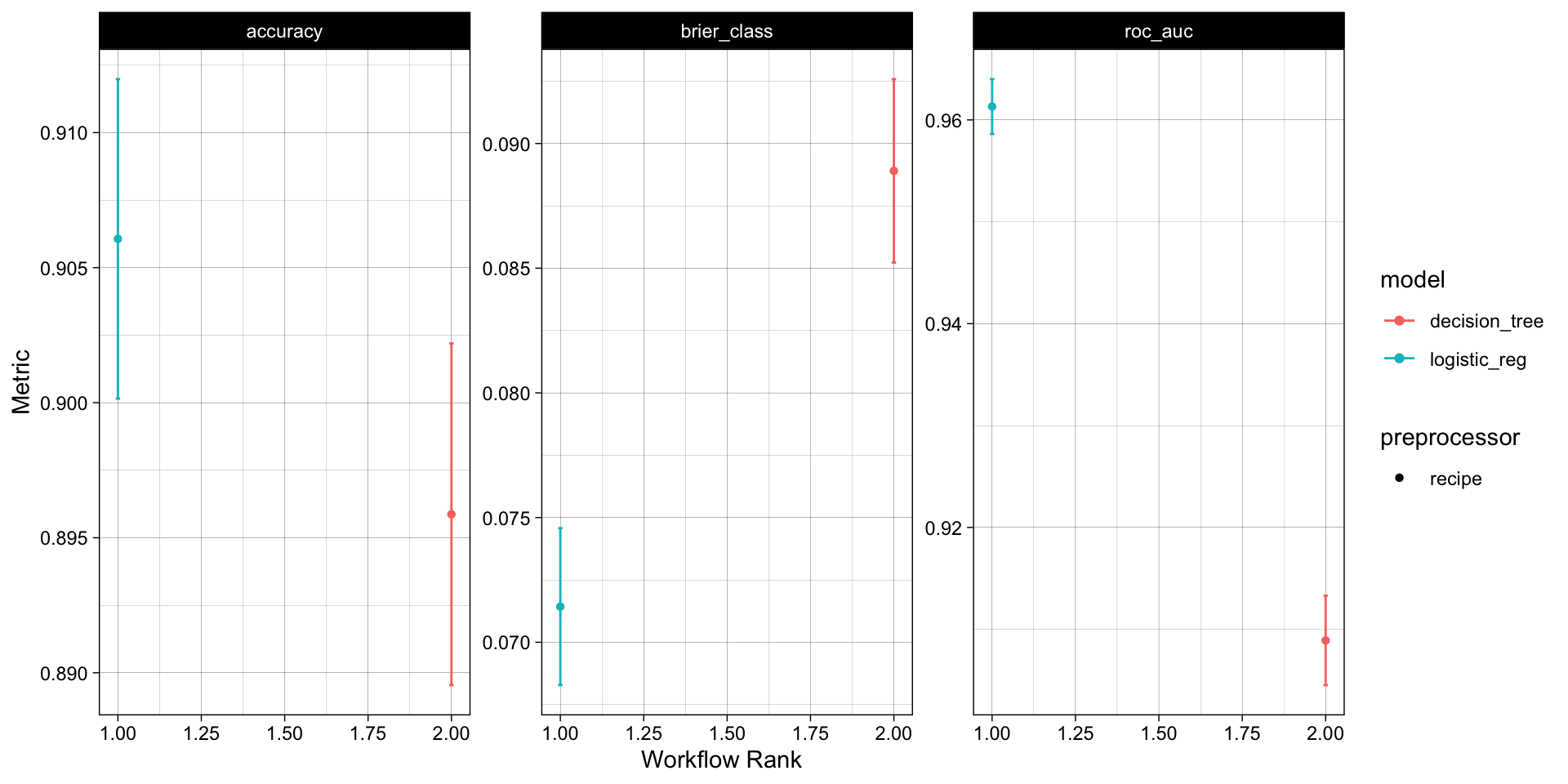
# Long list of results, ranked by accuracy
rank_results(wf_obj, 
            rank_metric = "accuracy", 
            select_best = TRUE)
#> # A tibble: 6 × 9
#>   wflow_id         .config .metric   mean std_err     n preprocessor model  rank
#>   <chr>            <chr>   <chr>    <dbl>   <dbl> <int> <chr>        <chr> <int>
#> 1 recipe_logistic… pre0_m… accura… 0.906  0.00360    10 recipe       logi…     1
#> 2 recipe_logistic… pre0_m… brier_… 0.0714 0.00191    10 recipe       logi…     1
#> 3 recipe_logistic… pre0_m… roc_auc 0.961  0.00164    10 recipe       logi…     1
#> 4 recipe_decision… pre0_m… accura… 0.896  0.00385    10 recipe       deci…     2
#> 5 recipe_decision… pre0_m… brier_… 0.0889 0.00224    10 recipe       deci…     2
#> 6 recipe_decision… pre0_m… roc_auc 0.909  0.00267    10 recipe       deci…     2

Overall, the logistic regression model appears to be the best model for this data set!

Note

Keep in mind: we compared these models out of the box, with no feature engineering, no hyperparameter tuning, and a single resampling scheme. Next week we’ll revisit this comparison once we can actually tune a model 👀

The whole game - status update

On Wednesday we’ll ask two things collect_metrics() can’t answer: which predictors did the model actually use (VIP) and is our 0.9-ish score honest (spatial cross-validation on autocorrelated data). Next week we’ll meet a bigger zoo of model families and learn to tune them.