Week 5
Beyond collect_metrics(): Interpretation & Spatial Resampling
Part 1: Which features mattered? ![]()

The vip package ![]()
vip is a lightweight, tidymodels-friendly interface for importance plots.
- Works with
parsnip/workflowobjects viaextract_fit_parsnip() - Supports model-specific importance for most engines
- Supports permutation importance for any model via
vip::vi_permute() vip()returns aggplot— easy to customize
Rebuild the forested pipeline ![]()
![]()


Exactly what we had last week — no new concepts yet:
set.seed(123)

forested_split <- initial_split(forested, strata = forested, prop = 0.8)
forested_train <- training(forested_split)
forested_test  <- testing(forested_split)

forested_folds <- vfold_cv(forested_train, v = 10, strata = forested)

forested_recipe <- recipe(forested ~ ., data = forested_train) |>
  step_impute_mean(all_numeric_predictors()) |>
  step_dummy(all_nominal_predictors()) |>
step_normalize(all_numeric_predictors())Model-specific VIP ![]()
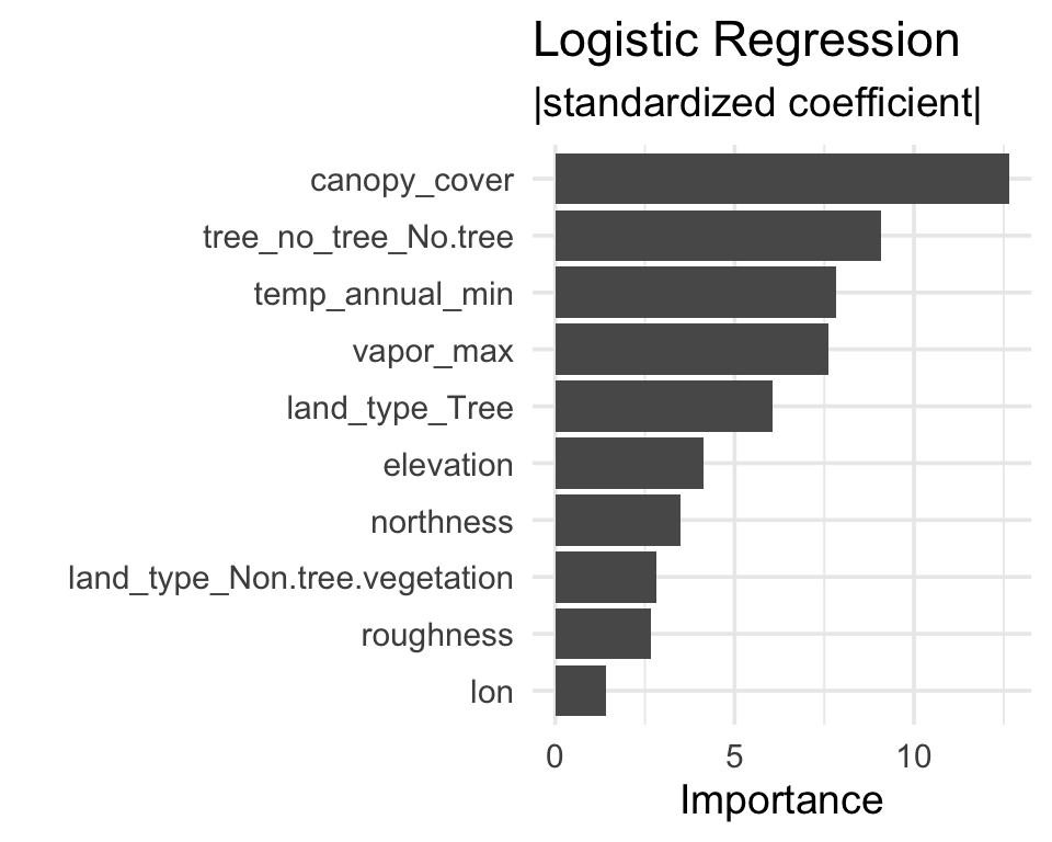
Logistic regression
Importance = absolute value of standardized coefficient.
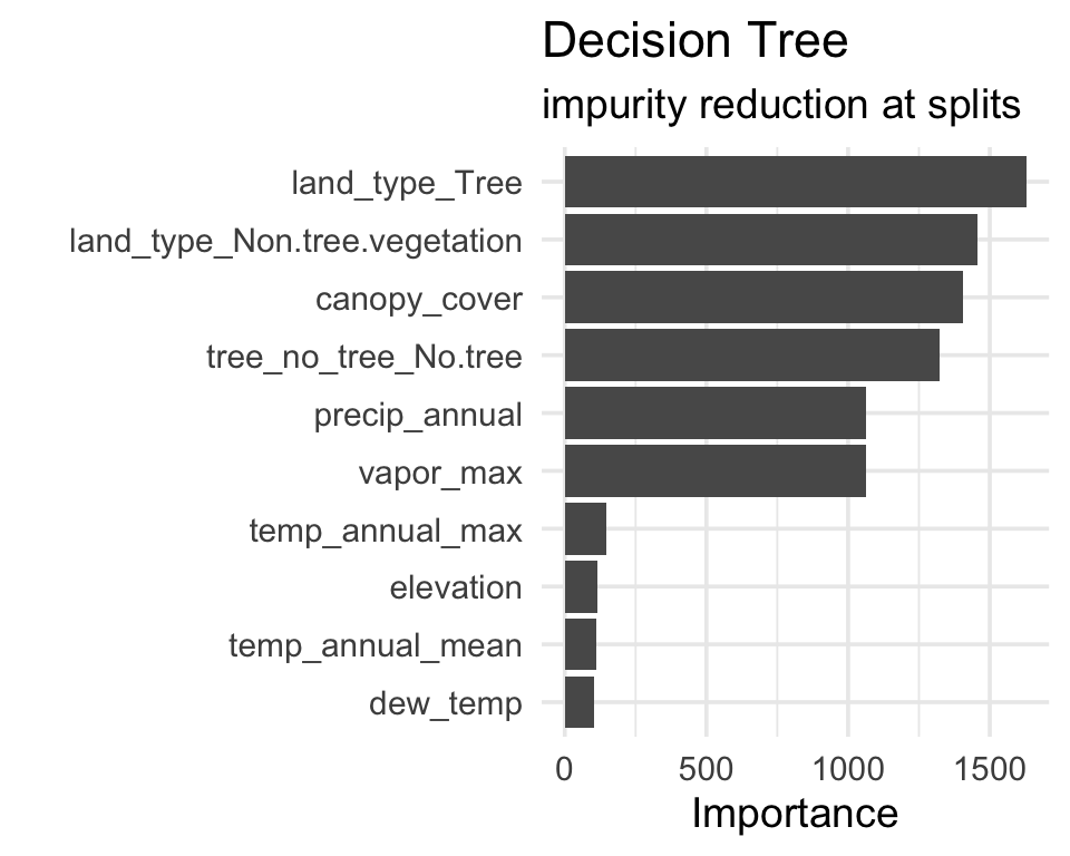
Agreement and disagreement ![]()
A feature’s rank in each model shows where they agree and where they diverge.
# Rank each model's features,
# keep the top 10 from either
ranks <- bind_rows(
  vi(extract_fit_parsnip(log_fit)) |>
    mutate(model = "logistic"),
  vi(extract_fit_parsnip(dt_fit)) |>
    mutate(model = "tree")
) |>
  group_by(model) |>
  mutate(rank = rank(-Importance)) |>
  group_by(Variable) |>
  filter(n() == 2, min(rank) <= 10)

ggplot(ranks,
       aes(model, rank, group = Variable)) +
  geom_line(color = "grey70") +
  geom_point(aes(color = model)) +
scale_y_reverse()- Flat lines → robust signal
- Swinging lines → model-specific
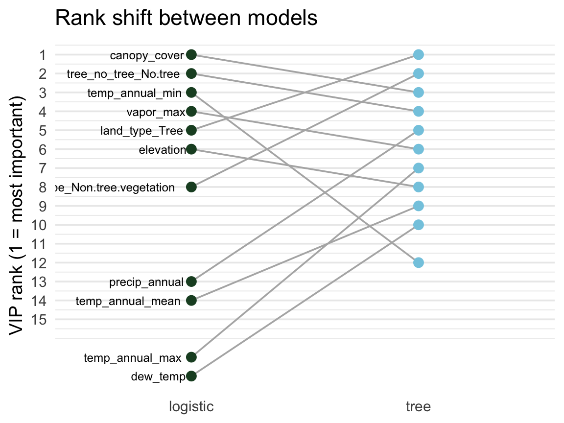
Tip
VIP is most informative across multiple models. Features important everywhere = probably real signal; features that matter only to one model type are often artifacts of how that model carves up the feature space.
Model-agnostic VIP (permutation) ![]()
Permutation importance works on any model — no internals required.
Algorithm:
- Fit the model.
- Compute a baseline metric (e.g., ROC AUC on a held-out set).
- For each predictor: randomly shuffle it, re-predict, recompute the metric.
- Importance = baseline metric − shuffled metric.
A predictor that, when scrambled, doesn’t hurt performance was not being used.
set.seed(321)

# A wrapper that returns the probability of the "Yes" class
pred_wrapper <- function(object, newdata) {
  predict(object, new_data = newdata, type = "prob")$.pred_Yes
}

vip::vi_permute(
  log_fit,
  train           = forested_train,
  target          = "forested",
  metric          = "roc_auc",
  reference_class = "Yes",
  pred_wrapper    = pred_wrapper,
  nsim            = 5
) |>
  vip::vip(num_features = 10) +
  labs(title = "Logistic regression — permutation importance")
Permutation importance is slow (shuffles + re-predicts once per feature per nsim), so you usually run it offline and save the result.
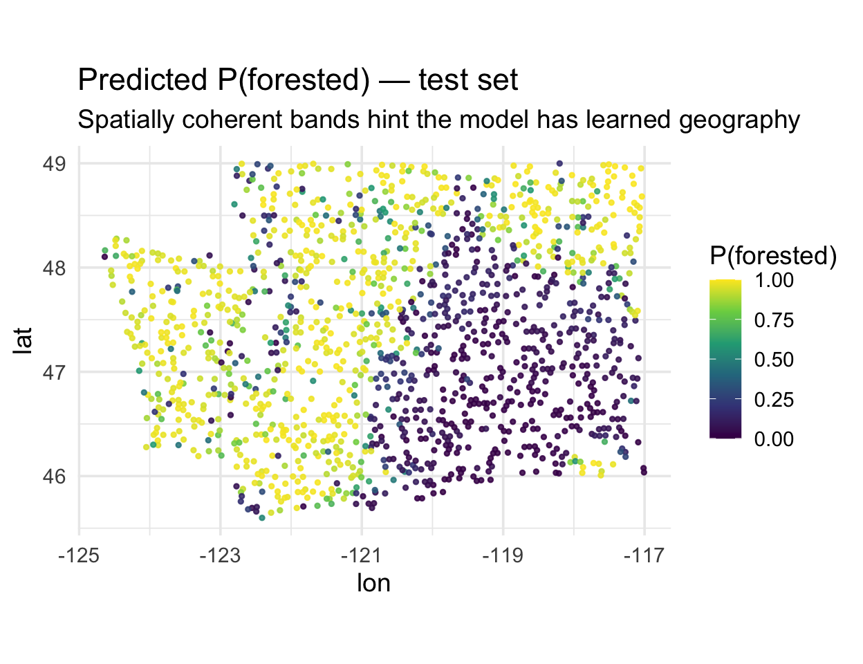
What does the model actually predict? ![]()

The forested dataset is spatial — map the predicted probability of forest for every test hexagon:
. . .
Notice the smooth spatial gradients. That’s informative — but also a warning sign: either (a) environmental drivers really do vary smoothly, or (b) the model is using location as a shortcut.
CV is supposed to tell us which.
Which predictors carry geography? ![]()

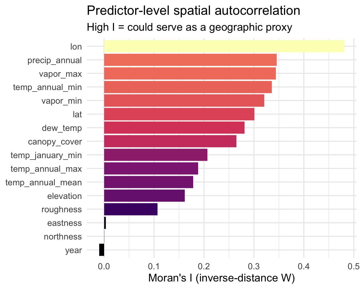
Before looking at residuals, let’s use Moran’s I on the predictors themselves. Features with high spatial autocorrelation are the ones a model could use as a shortcut for location:
library(ape)

set.seed(10)
samp <- slice_sample(forested_train, n = 400)
dmat <- as.matrix(dist(cbind(samp$lon, samp$lat)))
W <- 1 / dmat; diag(W) <- 0
W <- W / rowSums(W)

preds_I <- samp |>
  select(where(is.numeric), -forested) |>
  map_dfr(
    ~ tibble(I = Moran.I(.x, W)$observed),
    .id = "variable"
  ) |>
  arrange(desc(I))
Reading the ranking:
lon/lattop the list — by constructionprecip,vapor_*,temp_*are highly spatial (climate varies smoothly)eastness/northnessnear zero — aspect flips within a hillsideyear≈ 0 — it’s temporal, not spatial
Tip
Cross-reference this with your VIP plot. If your top-ranked features also sit near the top of this chart, they could be doing double duty as location encoders — a candidate for the spatial-CV check next.
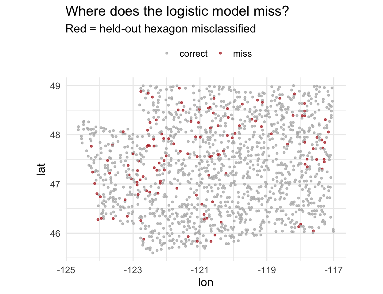
Residuals, mapped
. . .
Do you see clumps of red? That’s spatial autocorrelation in the residuals.
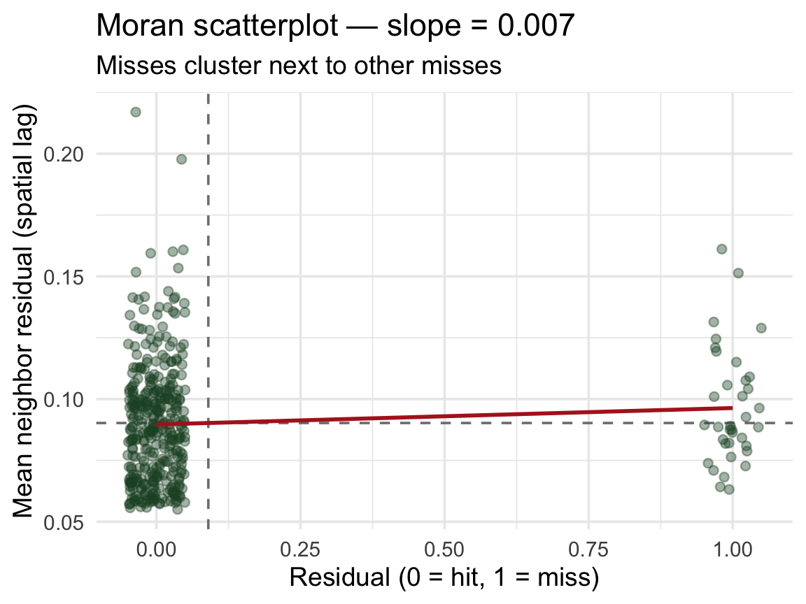
The Moran scatterplot ![]()

Moran’s I is the slope of a line through this scatterplot:
- x-axis: residual at a point
- y-axis: mean residual of its neighbors (spatial lag)
- upper-right / lower-left points → clustering
- diffuse cloud around zero → no spatial structure
. . .
The red line’s slope is Moran’s I. Positive slope → the model’s errors are geographically contagious → random CV is overstating performance.
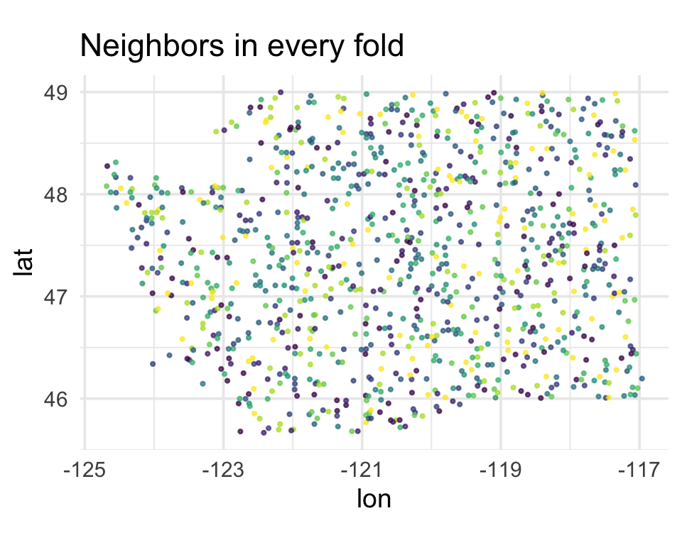
The leakage visualized
Every test point has a training point as a near neighbor. That’s the leakage.
Part 3: Spatial cross-validation ![]()
Enter spatialsample ![]()
The spatialsample package (a tidymodels extension) provides resampling schemes that respect geography.
| Function | How it splits |
|---|---|
spatial_block_cv() |
Tiles the area with a grid; assigns whole blocks to folds |
spatial_clustering_cv() |
k-means on coordinates, uses clusters as folds |
spatial_buffer_vfold_cv() |
Standard v-fold + removes a buffer of points around the held-out fold from training |
spatial_leave_location_out_cv() |
Leave out one named location (watershed, region, …) |
All produce familiar rset objects — they slot into fit_resamples() and workflow_map() unchanged.
📖 Reference: https://spatialsample.tidymodels.org/
Convert to an sf object ![]()

spatialsample needs spatial coordinates — we pass an sf object:
Note
We keep lon/lat as columns (remove = FALSE) so the model can still use them if it wants to — but conceptually that’s a smell, see Part 4.
Applying this to your data ![]()
Most real datasets don’t arrive as sf objects — they’re plain data frames with coordinate columns. Three things to watch for:
1. Column names vary. The forested data uses lon/lat, but your data might use longitude/latitude, gauge_lon/gauge_lat, X/Y, easting/northing. Pass whatever you have to coords = c(x, y):
2. The CRS must match the coordinates. Lon/lat in decimal degrees is EPSG:4326. If your data is projected (UTM, Albers, State Plane), use that EPSG code instead — otherwise your spatial blocks will be nonsense.
3. remove = FALSE is a modeling choice. Keeping the coordinate columns means your model can use them as predictors. Drop them in the recipe (step_rm(lon, lat)) if you want to force the model to rely on environmental features only.
Tip
Rule of thumb: always plot(st_geometry(your_sf)) once after conversion — if the points don’t land where you expect, the column order or CRS is wrong.
Spatial block CV ![]()
library(spatialsample)

set.seed(123)
forested_block <- spatial_block_cv(forested_sf, v = 10)

# Peek at the first few splits
print(forested_block, n = 3)
#> #  10-fold spatial block cross-validation
#> # A tibble: 10 × 2
#>   splits             id
#>   <list>             <chr>
#> 1 <split [5125/560]> Fold01
#> 2 <split [5114/571]> Fold02
#> 3 <split [5116/569]> Fold03
#> # ℹ 7 more rows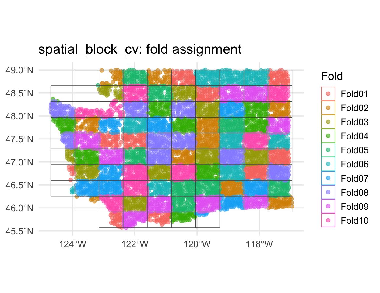
Compare the fold maps
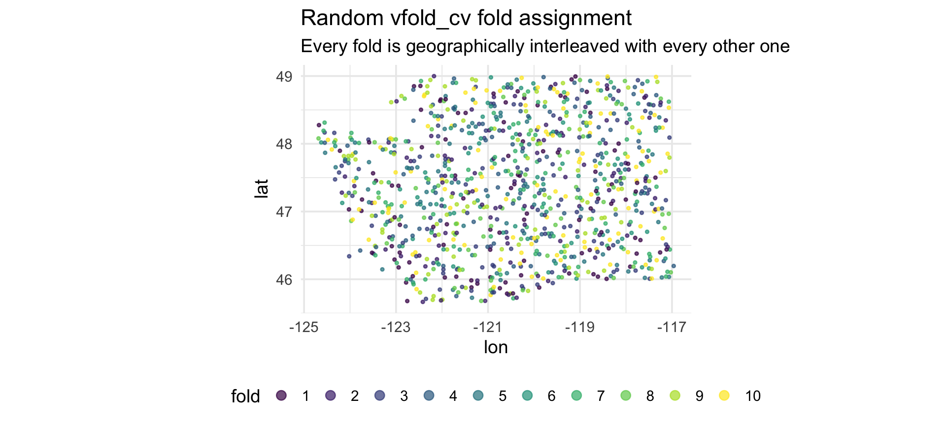
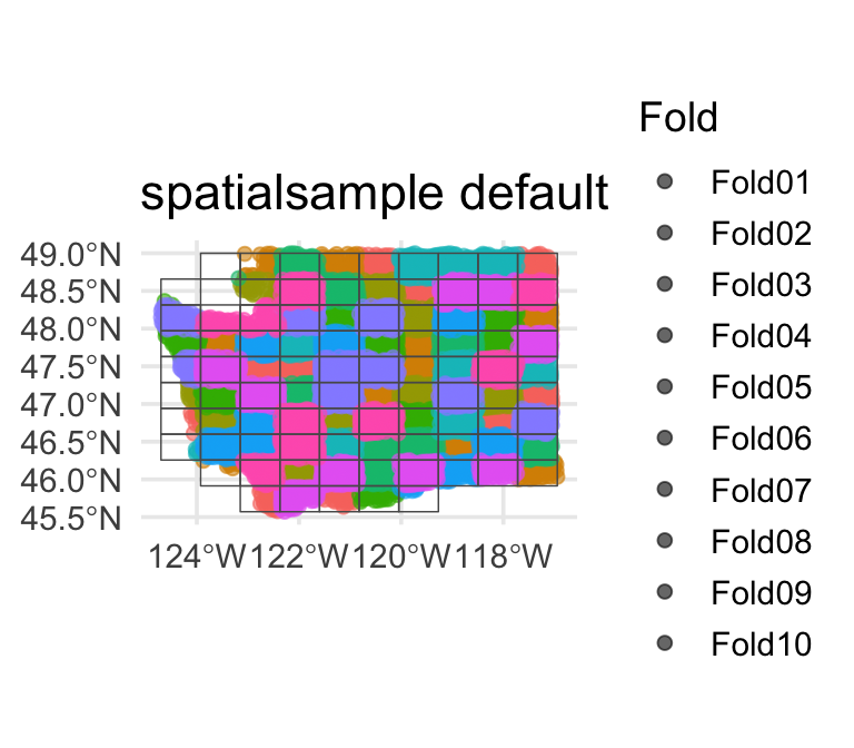
Random vfold_cv
Every fold contains points from every region of Washington. A held-out point has a training point next door.
spatial_block_cv
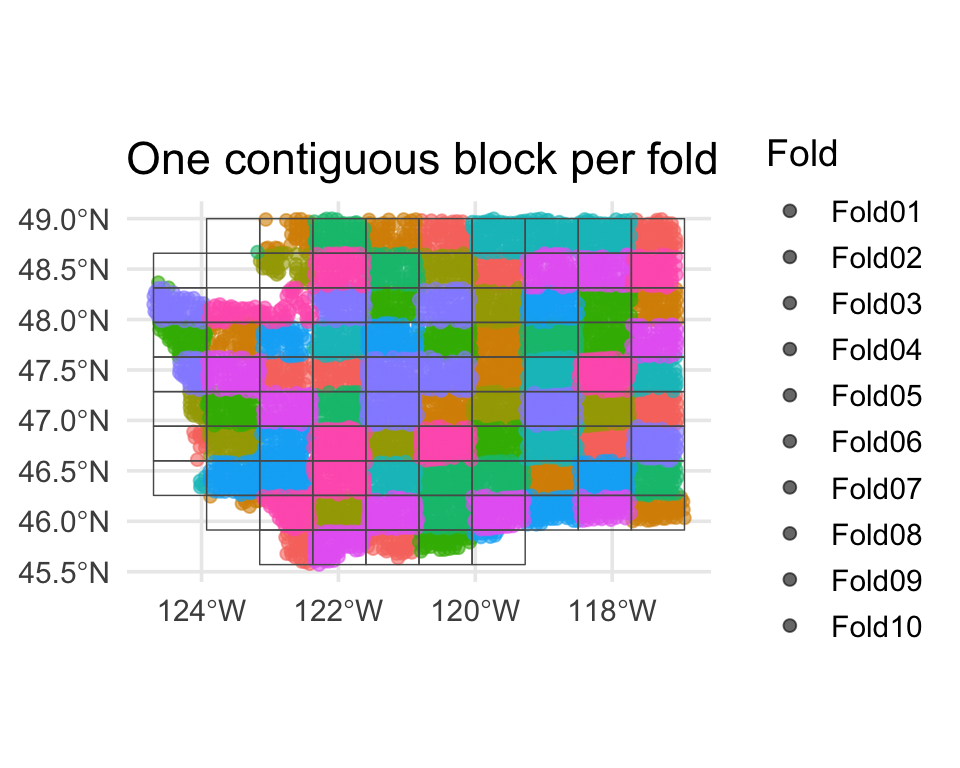
Each fold is a contiguous region. Holding it out simulates predicting somewhere the model has never seen.
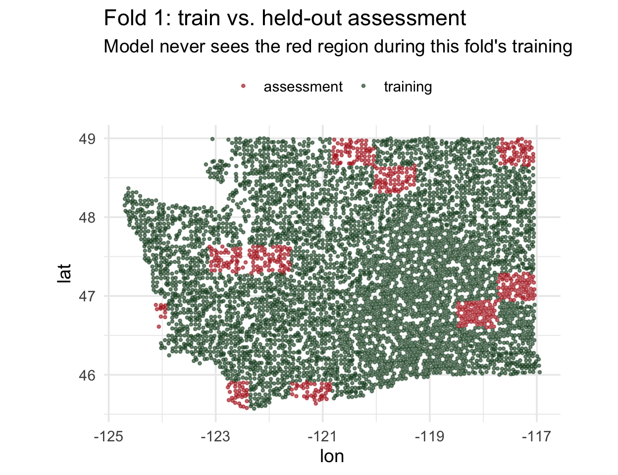
Zoom in on one fold ![]()
What does one spatial fold actually look like? Pull out fold 1 and plot its training and assessment sets:
. . .
This is the geometry random vfold_cv was quietly destroying: under random CV, those red points would have been surrounded by green ones.
Block size matters ![]()
spatial_block_cv() takes a cellsize argument (in CRS units). It controls the tile side length — and therefore how much spatial separation you actually get.
Small blocks (~0.1°)
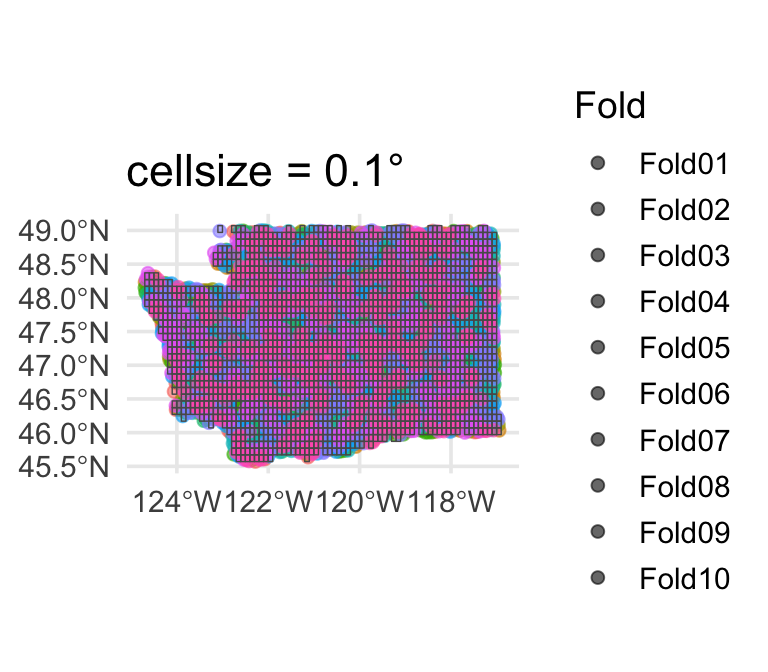
Too small — folds interleave again, essentially random CV.
Default (~0.5°)
Usually a reasonable starting point.
Large blocks (~1.5°)
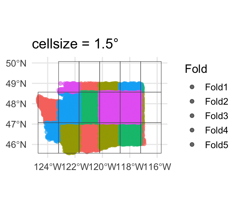
Very conservative — few effective folds, high fold-to-fold variance.
Tip
Rule of thumb: set cellsize to the spatial range of autocorrelation (from the variogram or Moran’s I distance bins). You want neighboring training points far enough from the test block that the model can’t just interpolate.
Re-fit the forested workflow ![]()
![]()


Identical to last week — only the resamples argument changes:
set.seed(2024)

cls_metrics <- metric_set(roc_auc, accuracy, brier_class)
ctrl        <- control_resamples(save_pred = TRUE)

log_rs_random  <- log_wf |>
  fit_resamples(resamples = forested_folds,  metrics = cls_metrics, control = ctrl)

log_rs_spatial <- log_wf |>
fit_resamples(resamples = forested_block, metrics = cls_metrics, control = ctrl)What a leaky model looks like ![]()
To make spatial leakage actually happen, we’d need a model that can only use geography. Fit a decision tree on lon + lat alone — no environmental predictors:
geo_recipe <- recipe(forested ~ lon + lat, data = forested_train) |>
  step_normalize(all_numeric_predictors())

geo_model <- decision_tree(tree_depth = 10, min_n = 3) |>
  set_engine("rpart") |> set_mode("classification")

geo_wf <- workflow() |> add_recipe(geo_recipe) |> add_model(geo_model)

set.seed(9)
geo_rs_random  <- fit_resamples(geo_wf, forested_folds, metrics = cls_metrics, control = ctrl)
geo_rs_spatial <- fit_resamples(geo_wf, forested_block, metrics = cls_metrics, control = ctrl)
#> # A tibble: 4 × 4
#> scheme .metric mean std_err
#> <chr> <chr> <dbl> <dbl>
#> 1 spatial_block_cv accuracy 0.788 0.0163
#> 2 vfold_cv (random) accuracy 0.834 0.00381
#> 3 spatial_block_cv roc_auc 0.796 0.0182
#> 4 vfold_cv (random) roc_auc 0.839 0.00511Warning
Now the gap shows up. Random CV still gives the tree high marks — every held-out hexagon has a neighbor from a different fold to interpolate from. Spatial CV drops ~0.05 AUC because whole regions of Washington are held out and the model has no other signal to fall back on. That gap is spatial leakage — caught red-handed.
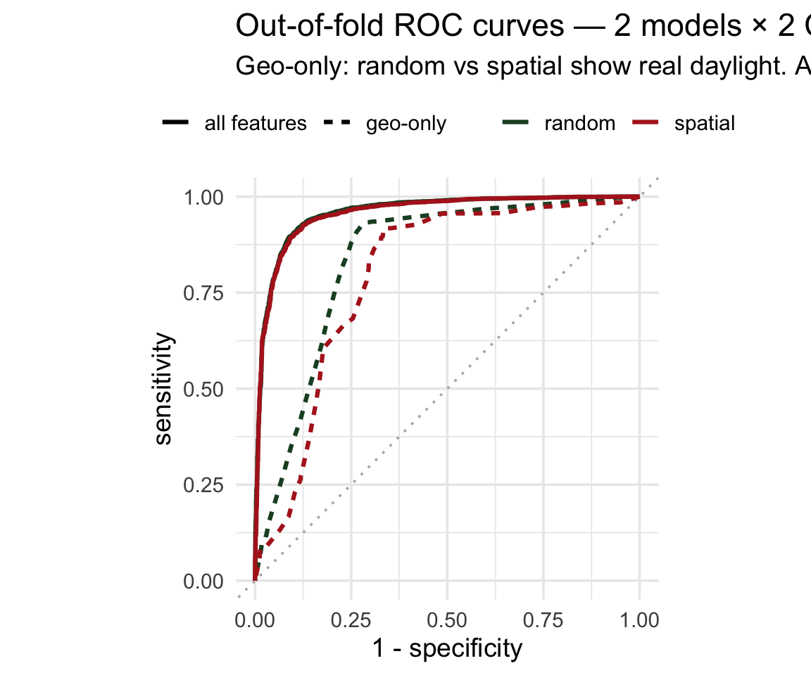
ROC curves: all four fits overlaid ![]()

Overlay the out-of-fold predictions from each model × CV scheme:
roc_data <- bind_rows(
  collect_predictions(log_rs_random)  |>
    mutate(model = "all features",
           scheme = "random"),
  collect_predictions(log_rs_spatial) |>
    mutate(model = "all features",
           scheme = "spatial"),
  collect_predictions(geo_rs_random)  |>
    mutate(model = "geo-only",
           scheme = "random"),
  collect_predictions(geo_rs_spatial) |>
    mutate(model = "geo-only",
           scheme = "spatial")
) |>
  group_by(model, scheme) |>
  roc_curve(truth = forested, .pred_Yes)

ggplot(roc_data,
       aes(1 - specificity, sensitivity,
           color = scheme, linetype = model)) +
  geom_path(linewidth = 1.1) +
  coord_equal()
The all-features pair is on top of each other — no leakage to find. The geo-only pair shows visible daylight between random and spatial — the spatial curve sagging is what leakage looks like.
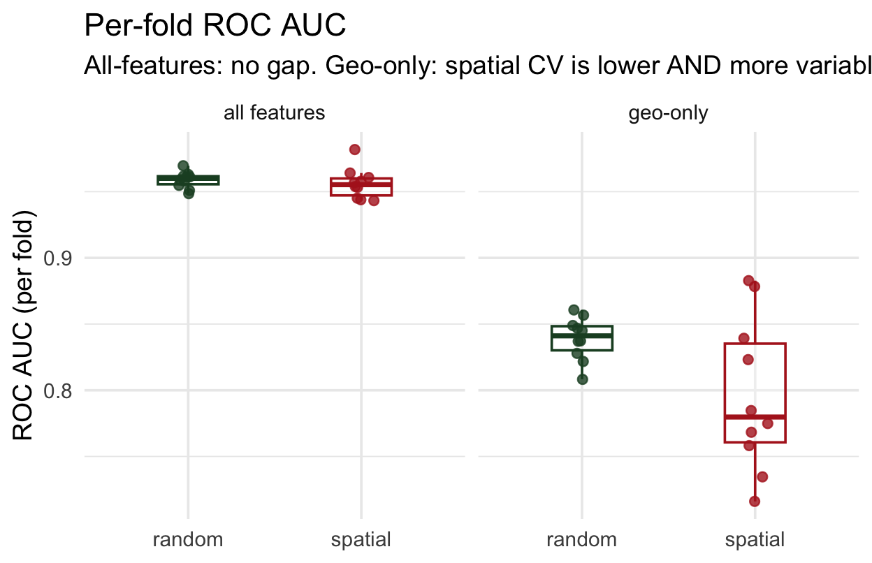
It’s not just lower — it’s more variable ![]()
The mean hides the story. Pull per-fold metrics for both models × both schemes:
per_fold <- bind_rows(
  collect_metrics(log_rs_random,  summarize = FALSE) |>
    mutate(model = "all features", scheme = "random"),
  collect_metrics(log_rs_spatial, summarize = FALSE) |>
    mutate(model = "all features", scheme = "spatial"),
  collect_metrics(geo_rs_random,  summarize = FALSE) |>
    mutate(model = "geo-only",     scheme = "random"),
  collect_metrics(geo_rs_spatial, summarize = FALSE) |>
    mutate(model = "geo-only",     scheme = "spatial")
) |> filter(.metric == "roc_auc")

ggplot(per_fold,
       aes(interaction(model, scheme), .estimate,
           color = scheme)) +
  geom_boxplot() +
  geom_jitter(width = 0.08)
All-features: both CV schemes give tight, near-identical distributions → no leakage. Geo-only: spatial folds show lower mean AND wider spread — the model’s performance depends heavily on which region you hold out.
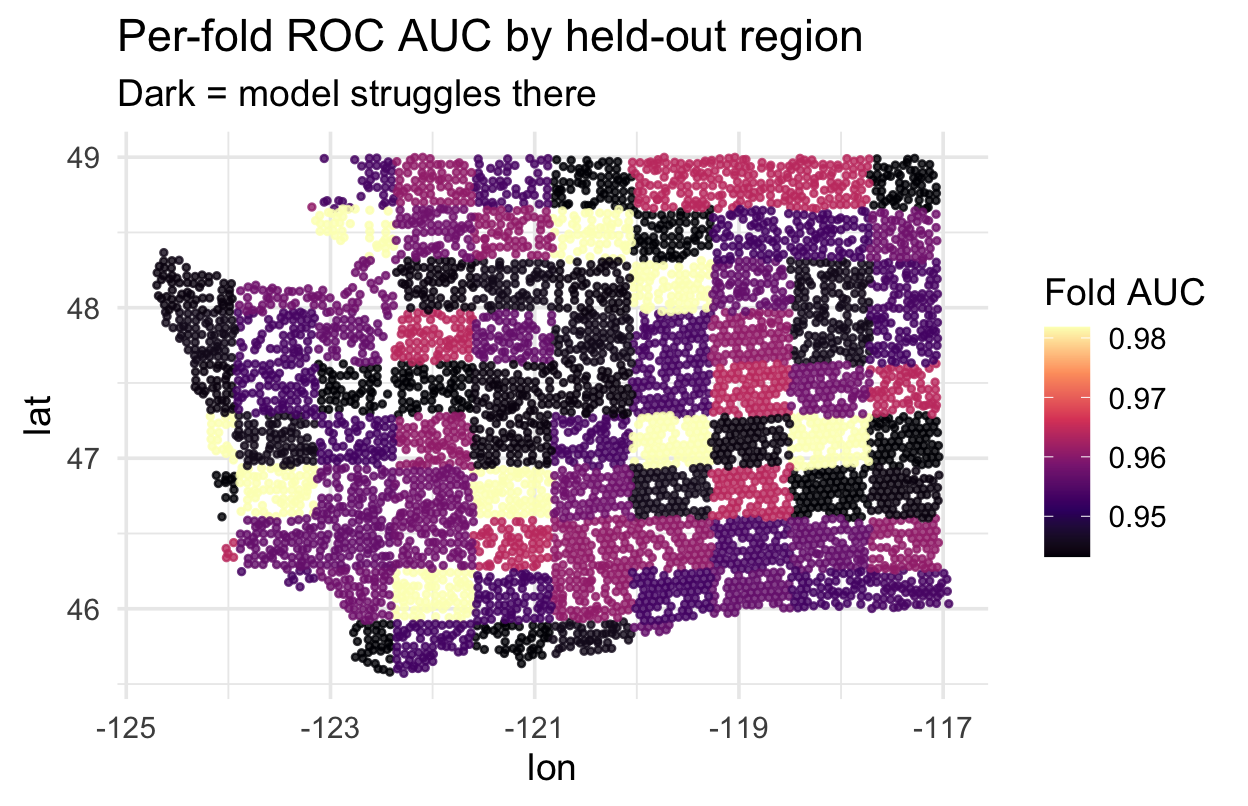
Where does spatial CV struggle? ![]()
Each spatial fold’s held-out region has a location. Map each fold’s AUC to see which regions are hardest to predict:
fold_auc <- collect_metrics(
    log_rs_spatial, summarize = FALSE) |>
  filter(.metric == "roc_auc") |>
  select(id, fold_auc = .estimate)

# join each fold's AUC back to its
# held-out coordinates (see repo)

ggplot(fold_locations,
       aes(lon, lat, color = fold_auc)) +
  geom_point() +
  scale_color_viridis_c(option = "magma")
Regions where AUC is lowest are where your model has the least transferable signal — a scientific finding telling you where to invest more training data or features.
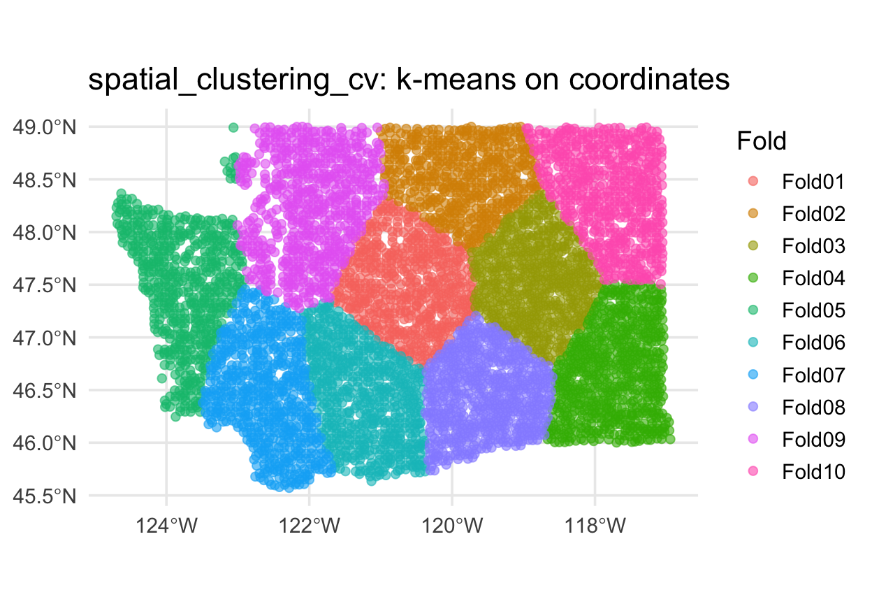
Alternative: spatial_clustering_cv ![]()
When blocks don’t fit your data (e.g., irregularly shaped study regions), cluster-based folds are often better:
Alternative: buffered v-fold ![]()
What if you want random folds but guarantee no training point is within, say, 10 km of a test point?
- Each training set has points within
bufferof held-out points removed - Preserves fold size randomness; enforces a minimum spatial gap
- Good compromise when blocks are too coarse but random CV is too leaky
Warning
buffer is expressed in the units of the CRS. Buffers on geographic (lon/lat) CRSs give meaningless results — always transform to a projected CRS first.
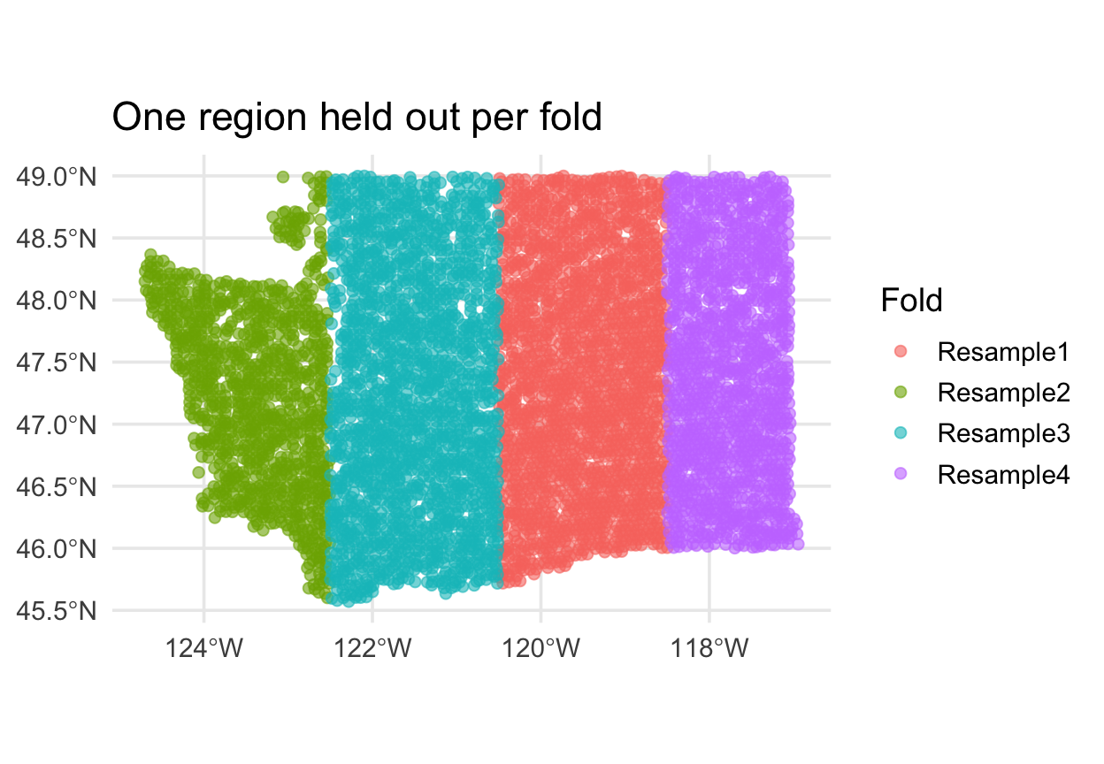
Alternative: leave-location-out CV ![]()
For water resources, the natural unit is usually a watershed, gauge basin, or ecoregion — not a square block. spatial_leave_location_out_cv() holds out one named group at a time:
Each fold trains on 3 regions and predicts the 4th — answers “could I predict eastern WA from coastal WA?”, which vfold_cv can’t. In your project, swap region for HUC8, gauge basin, or climate zone.
The 2×2 comparison
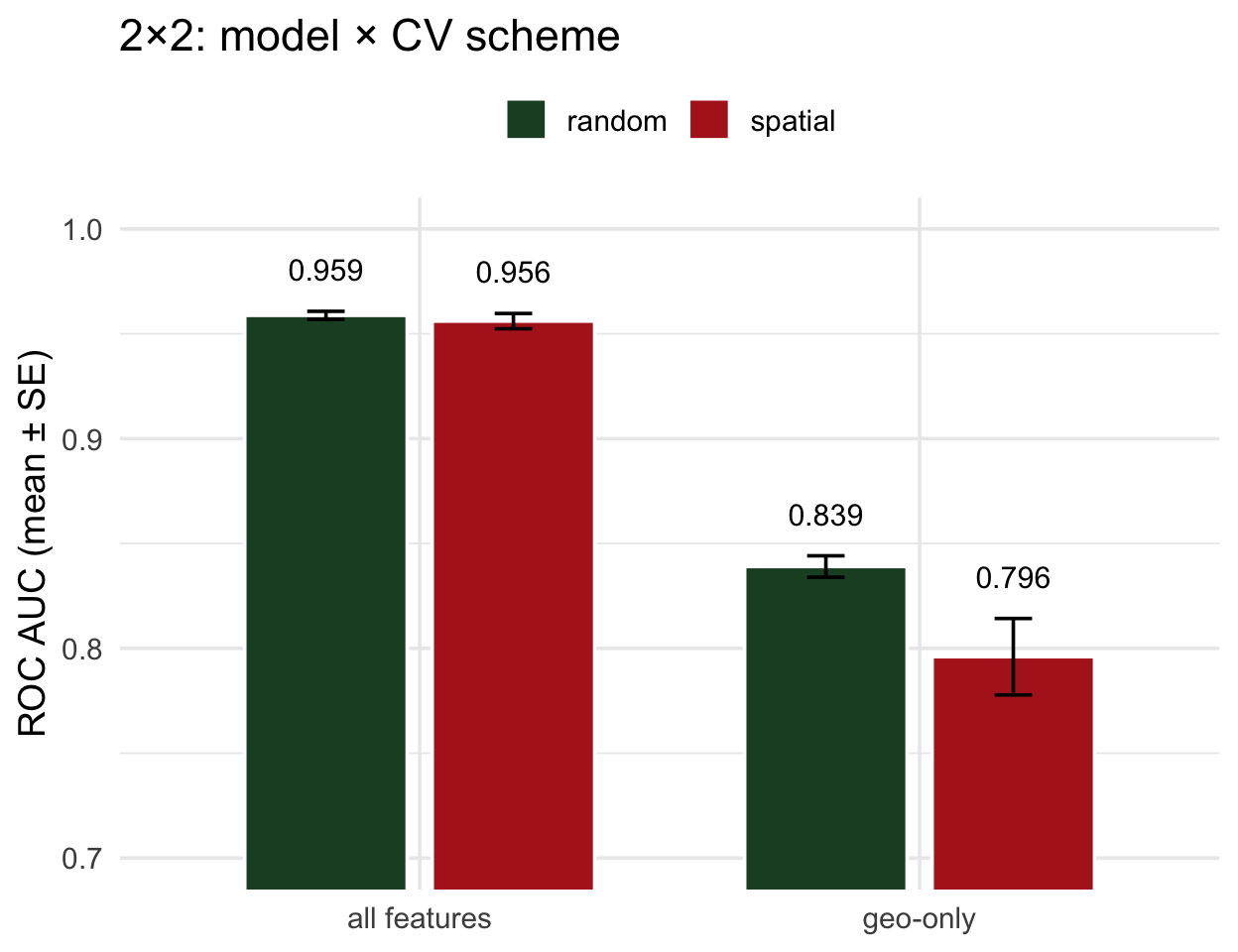
- All features, random ≈ spatial → no leakage; random CV was telling the truth
- Geo-only, random ≫ spatial → the gap is the leakage
- The diagnostic is the within-model gap, not the between-model one
. . .
Read it this way: compare the two bars within each model. Equal = trust the number. Unequal = your model’s random-CV score is inflated by exactly that much.
The same idea in regression ![]()
Every example above used classification (forested: Yes/No) — but the same leakage story applies to regression. You just swap the metric.
Pretend we’re predicting log mean streamflow (logQmean) from basin attributes for CAMELS gauges — a spatial regression problem. The 2×2 would be built the same way:
- Classification: higher ROC AUC = better → spatial CV usually lowers AUC
- Regression: higher R² = better → spatial CV usually lowers R²
- Regression: lower RMSE = better → spatial CV usually raises RMSE
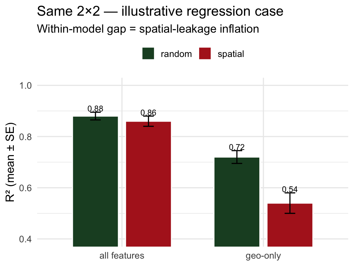
The within-model gap (random vs spatial) is the diagnostic — just on a regression metric instead of AUC.
Important
For your lab: CAMELS basins have gauge_lon/gauge_lat. Random vfold_cv on CAMELS is the regression version of the story above. Build a spatial_block_cv next to it and report both — the delta is the honest cost of generalization.