Week 6

Machine Learning Part 2

Introduction

Machine learning (ML) is widely used in environmental science for tasks such as land cover classification, climate modeling, and species distribution prediction. This lecture explores five common ML model families available through the tidymodels framework in R, applied to the forested dataset we met last week.

Linear Regression
Logistic Regression
Trees
- Decision Tree
- Random Forest
- Boosted Trees
Support Vector Machines
Neural Networks

By the end of today you will be able to…

Distinguish classification from regression modes and pick the right one for an environmental question
Specify seven major model families with parsnip (linear, logistic, tree, random forest, boosted trees, SVM, neural network)
Read and interpret classification metrics from a confusion matrix: accuracy, sensitivity, specificity, ROC AUC, Brier score
Compare models systematically using workflow_set() over cross-validation folds

Running example: continuing the forested dataset from last week — can we predict whether a 6,000-acre hexagon in Washington is forested?

Classification vs. Regression

In tidymodels, a model’s mode tells the engine what kind of outcome it’s predicting:

Classification → Predict a categorical outcome (discrete classes).

Regression → Predict a numeric outcome (a continuous value).

Many of the same model families (trees, SVMs, neural networks, …) can do either — you pick the mode with set_mode().

Classification Models

Goal: Categorize phenomena into discrete classes.

Examples:

✅ Land Cover Classification (Forest, Urban, Water, Agriculture)
✅ Flood Risk Assessment (High, Medium, Low)
✅ Drought Severity Levels (No Drought, Moderate, Severe)
✅ Wildfire Prediction (Fire vs. No Fire)
✅ Species Identification (Bird species, Plant types)

Common Algorithms:

Decision Trees
Random Forest
Support Vector Machines (SVM)
Neural Networks (for remote sensing & image analysis)
K-Nearest Neighbors (KNN)

Regression Models

Goal: Estimate continuous environmental variables.

Examples:

📈 Streamflow Forecasting (Predict river discharge over time)
🌡️ Temperature Projections (Future temperature changes under climate scenarios)
☔ Precipitation Forecasting (Rainfall estimates for flood preparedness)
📊 Air Quality Index Prediction (Forecast pollution levels)

Common Algorithms:

Linear & Multiple Regression
Random Forest Regression
Long Short-Term Memory (LSTM) Neural Networks (for time series forecasting)

Choosing the Right Model

Use classification if: You need to categorize environmental states (e.g., classifying land use changes).
Use regression if: You need to estimate a continuous environmental value (e.g., predicting flood levels).
Use hybrid approaches if: You need to classify and estimate (e.g., classifying drought severity and predicting future water availability).

Model Selection Considerations

Choosing an ML algorithm (model) depends on:

Dataset Size: e.g. Large datasets benefit from ensemble methods like Random Forest and XGBoost.
Feature Complexity: e.g. SVM works well for high-dimensional data.
Interpretability Needs: e.g. Decision trees and LASSO regression provide intuitive insights.
Computation Constraints: e.g. GLM and Decision Trees are efficient compared to XGBoost.
Data: Variance, linearity, dimensionality

Load Required Libraries

library(tidyverse)
library(tidymodels)
library(forested)
library(flextable)

Data Preparation

We will use the forested dataset for classification. Each row is a 6,000-acre hexagon in Washington state with an on-the-ground forested label ("Yes"/"No") and 18 remotely-sensed predictors (elevation, climate summaries, vegetation indices, etc.).

set.seed(123)
forested_split <- initial_split(forested, strata = forested)
forested_train <- training(forested_split)
forested_test  <- testing(forested_split)
forested_folds <- vfold_cv(forested_train, v = 10)

# Feature Engineering: Classification
forested_recipe <- recipe(forested ~ ., data = forested_train) |>
  step_impute_mean(all_numeric_predictors()) |>
  step_dummy(all_nominal_predictors()) |>
  step_normalize(all_numeric_predictors())

Machine Learning Specifications in `tidymodels`

Unified Interface for ML Models

The parsnip package is a part of the tidymodels framework
It provides a consistent interface for specifying models across many different algorithms
The combination of a specification, mode, and engine is called a model
Let’s look at the parsnip documentation!

Metric vocabulary — what `collect_metrics()` will show us

Every example below ends with a collect_metrics() call. For classification models the default output is three metrics you should know before reading them:

Metric	What it measures	Range	Good value
accuracy	Fraction of predictions that match the truth	0–1	higher
roc_auc	Probability the model ranks a true positive above a true negative at any threshold (separation)	0–1	higher (>0.8 good)
brier_class	Mean squared error between predicted probability and outcome (calibration)	0–1	lower (<0.25 acceptable)

We’ll unpack each — plus sensitivity, specificity, and the confusion matrix — after the model zoo.

Note

Regression models default to rmse, rsq, mae instead — covered in the Regression Metrics section.

What are hyperparameters?

Hyperparameters are settings that control the learning process of a model.
They are set before training and affect the model’s performance.
Hyperparameters can be tuned to optimize the model’s predictive power.
More on model tuning later in today’s lecture!

Today’s model zoo, at a glance

`parsnip` function	Family	Typical strength	Typical weakness	Key hyperparameters
`linear_reg()`	Linear	Fast, interpretable	Assumes linearity	`penalty`, `mixture`
`logistic_reg()`	GLM (classification)	Probabilities + interpretable coefs	Linear decision boundary	`penalty`, `mixture`
`decision_tree()`	Tree	Visual, handles non-linearity	Overfits, unstable	`tree_depth`, `min_n`, `cost_complexity`
`rand_forest()`	Tree ensemble (bagging)	Robust, little tuning needed	Slower, less interpretable	`trees`, `mtry`, `min_n`
`boost_tree()`	Tree ensemble (boosting)	Often top accuracy on tabular data	Tuning-sensitive, risk of overfit	`trees`, `learn_rate`, `min_n`, `mtry`
`svm_poly()` / `svm_rbf()`	Margin-based	High-dim, small-N friendly	Slow at scale, needs scaling	`cost`, `degree`, `rbf_sigma`
`mlp()`	Neural network	Learns complex non-linearities	Data-hungry, opaque	`hidden_units`, `penalty`, `epochs`

We’ll walk through each family below — keep this table handy; we won’t re-derive each row.

Linear Regression

Linear regression is a fundamental statistical method used for modeling the relationship between a dependent variable and one or more independent variables. It is widely used in environmental science for tasks such as predicting species distribution, estimating climate variables, and modeling ecosystem dynamics.

Components of Linear Regression

Dependent Variable (Y): The variable to be predicted.
Independent Variables (X): Features that influence the dependent variable.
Regression Line: Represents the relationship between X and Y.
Residuals: Differences between predicted and actual values.

Linear Regression in `tidymodels`

Specification

linear_reg()

#> Linear Regression Model Specification (regression)
#> 
#> Computational engine: lm

engines & modes

show_engines("linear_reg") |> 
  mutate(specification = "linear_reg") |> 
  flextable()

engine	mode	specification
lm	regression	linear_reg
glm	regression	linear_reg
glmnet	regression	linear_reg
stan	regression	linear_reg
spark	regression	linear_reg
keras	regression	linear_reg
brulee	regression	linear_reg
quantreg	quantile regression	linear_reg

Example

Warning

This example predicts elevation from the other columns — it’s a syntactic demo of parsnip’s regression mode, not a meaningful scientific model. In a real regression problem you’d pick an outcome that represents what you actually want to estimate.

# penalty and mixture are available when engine = "glmnet" (regularized regression)
lm_mod <- linear_reg(mode = "regression", engine = "lm")

workflow() |>
  add_formula(elevation ~ .) |>
  add_model(lm_mod) |>
  fit_resamples(resamples = forested_folds) |>
  collect_metrics()
#> # A tibble: 2 × 6
#>   .metric .estimator   mean     n std_err .config        
#>   <chr>   <chr>       <dbl> <int>   <dbl> <chr>          
#> 1 rmse    standard   82.9      10 1.33    pre0_mod0_post0
#> 2 rsq     standard    0.971    10 0.00120 pre0_mod0_post0

Logistic Regression

Logistic Regression is used for binary classification tasks. It models the probability that an observation belongs to a category using the logistic (sigmoid) function. Unlike linear regression, which predicts continuous values, logistic regression predicts probabilities and applies a decision threshold to classify outcomes.

Components of Logistic Regression

Sigmoid Function: Squashes any real number into a probability between 0 and 1. A large positive score → near 1 (“yes”); a large negative score → near 0 (“no”). (top plot: the S-curve)
Decision Boundary: Once we have probabilities, we pick a cutoff (default 0.5) to assign a class. Everything above → “Yes”, below → “No”. (top plot: the dashed line separating the two groups)
Log-Loss (Binary Cross-Entropy): The model’s training objective — penalizes confident wrong predictions harshly. Lower is better. (bottom plot: loss falling as training progresses)
Regularization (L1 and L2): A penalty added to the loss that shrinks large coefficients toward zero — prevents the model from over-relying on any single feature.

Variants of Logistic Regression

Binary Logistic Regression: Used when the target variable has two classes (e.g., forested vs. not).
Multinomial Logistic Regression: Extends logistic regression to multiple classes without assuming ordering.
Ordinal Logistic Regression: Handles multi-class classification where order matters (e.g., rating scales).

Building a Logistic Regression Model

Constructing a Logistic Regression Model involves:

Defining feature (X) and target variable (y).
Applying the sigmoid function to map predictions to probabilities.
Using a loss function (log-loss) to optimize model weights.
Updating weights iteratively via gradient descent.

Hyperparameters in Logistic Regression

penalty (λ): Strength of regularization — how much large coefficients are penalized. Higher → simpler model, less overfitting but potentially underfit. Lower → model fits training data more closely, risk of overfitting. Tuned on a log scale (e.g., 10⁻⁵ to 1).
mixture (α): Blend of L1 (lasso) and L2 (ridge) regularization. 0 → pure ridge (shrinks all coefficients, keeps all features). 1 → pure lasso (drives some coefficients to exactly zero, effectively removing features). Values between 0–1 blend both behaviors.

Logistic Regression in `tidymodels`

Specification

logistic_reg()

#> Logistic Regression Model Specification (classification)
#> 
#> Computational engine: glm

engines & modes

show_engines('logistic_reg') |> 
  mutate(specification = "logistic_reg") |> 
  flextable()

engine	mode	specification
glm	classification	logistic_reg
glmnet	classification	logistic_reg
LiblineaR	classification	logistic_reg
spark	classification	logistic_reg
keras	classification	logistic_reg
stan	classification	logistic_reg
brulee	classification	logistic_reg

Example

log_model <- logistic_reg(penalty = 0.01, mixture = 0) |>
  set_engine("glmnet") |>
  set_mode('classification')

workflow() |>
  add_recipe(forested_recipe) |>
  add_model(log_model) |> 
  fit_resamples(resamples = forested_folds) |>
  collect_metrics()
#> # A tibble: 3 × 6
#>   .metric     .estimator   mean     n std_err .config        
#>   <chr>       <chr>       <dbl> <int>   <dbl> <chr>          
#> 1 accuracy    binary     0.898     10 0.00392 pre0_mod0_post0
#> 2 brier_class binary     0.0778    10 0.00230 pre0_mod0_post0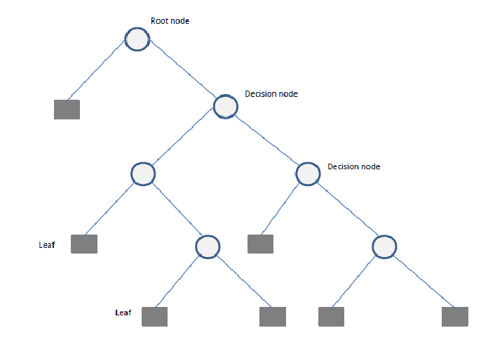
#> 3 roc_auc     binary     0.957     10 0.00211 pre0_mod0_post0

Decision Tree

A Decision Tree is a flowchart-like structure used for decision-making and predictive modeling. It consists of nodes representing decisions, branches indicating possible outcomes, and leaf nodes that represent final classifications or numerical outputs. Decision Trees are widely used in both classification and regression tasks.

Components of a Decision Tree

Root Node: The starting point representing the entire dataset.
Decision Nodes: Intermediate nodes where a dataset is split based on a feature.
Splitting: The process of dividing a node into sub-nodes based on a feature value.
Pruning: The process of removing unnecessary branches to avoid overfitting.
Leaf Nodes: The terminal nodes that provide the final output (class label or numerical prediction).

Building a Decision Tree

Constructing a Decision Tree involves:

Selecting the best feature(s) to split the data.
Splitting the data into subsets.
Repeating this process recursively until stopping criteria (e.g., depth, minimum samples per leaf) are met.
Pruning the tree if necessary to reduce overfitting.

Splitting Criteria

Several criteria can be used to determine the best split:
- Gini Impurity: Measures the impurity of a node, used in Classification and Regression Trees (CART).
- Entropy (Information Gain): Measures the randomness in a dataset.
- Mean Squared Error (MSE): Used for regression trees to minimize variance within nodes.

Hyperparameters in Decision Trees

cost_complexity (Cp): Penalty applied to each additional split during pruning. Higher → more pruning, simpler tree, less overfitting. Lower → tree grows more freely and fits training data more closely. Default is 0.01; setting near 0 allows full growth.
tree_depth: Maximum number of splits from root to leaf. Higher → tree can capture more complex patterns. Lower → simpler, more generalizable tree. Depth 1 creates a single-split “stump.” Typical range: 3–15.
min_n: Minimum number of observations required in a node before attempting a split. Higher → fewer, larger leaves (acts as regularization). Lower → finer-grained splits that may overfit noise.

Decision Tree using tidymodels

Specification

decision_tree()

#> Decision Tree Model Specification (unknown mode)
#> 
#> Computational engine: rpart

engines & modes

show_engines('decision_tree') |> 
  mutate(specification = "decision_tree") |> 
  flextable()

engine	mode	specification
rpart	classification	decision_tree
rpart	regression	decision_tree
C5.0	classification	decision_tree
spark	classification	decision_tree
spark	regression	decision_tree

Example

dt_model <- decision_tree(cost_complexity = 0.01, tree_depth = 10, min_n = 3) |>
  set_engine("rpart") |>
  set_mode('classification')

workflow() |>
  add_recipe(forested_recipe) |>
  add_model(dt_model) |>
  fit_resamples(resamples = forested_folds) |>
  collect_metrics()
#> # A tibble: 3 × 6
#>   .metric     .estimator   mean     n std_err .config        
#>   <chr>       <chr>       <dbl> <int>   <dbl> <chr>          
#> 1 accuracy    binary     0.898     10 0.00337 pre0_mod0_post0
#> 2 brier_class binary     0.0878    10 0.00287 pre0_mod0_post0
#> 3 roc_auc     binary     0.908     10 0.00391 pre0_mod0_post0

Tip

Notice the pattern: recipe → model → fit_resamples → collect_metrics. It’s going to repeat for every model below. We’ll generalize this repetition with workflow_set() at the end so you don’t write the same four lines six times.

Random Forest

Random Forest is an ensemble learning method that constructs multiple decision trees and aggregates their predictions to improve accuracy and reduce overfitting. It can be used for both classification and regression tasks.

Components of a Random Forest

Multiple Decision Trees: The fundamental building blocks.
Bootstrap Sampling: Randomly selects subsets of data to train each tree.
Feature Subsetting: Uses a random subset of features at each split to improve diversity among trees.
Aggregation (Bagging): Combines the outputs of individual trees through voting (classification) or averaging (regression).

Building a Random Forest

Constructing a Random Forest involves:

Creating multiple bootstrap samples from the dataset.
Training a decision tree on each bootstrap sample using a random subset of features.
Aggregating predictions from all trees to produce the final output.

Hyperparameters in Random Forest

trees: Number of trees in the ensemble. More trees → more stable, reliable predictions. Diminishing returns beyond ~500. Unlike depth, adding trees almost never hurts — it’s mainly a compute budget question. Start with 500–1000.
min_n: Minimum observations needed before a node can split. Higher → shallower, more regularized trees with larger leaves. Lower → deeper trees that fit training data more closely. Acts as implicit depth control across all trees.
mtry: Number of features randomly considered at each split. Lower → more diverse, decorrelated trees (often better ensemble performance). Higher → each tree is individually stronger but trees become more similar. Default is √p (classification) or p/3 (regression), where p = number of predictors.

Random Forest Implementation using Tidymodels

Specification

rand_forest()

#> Random Forest Model Specification (unknown mode)
#> 
#> Computational engine: ranger

engines & modes

show_engines('rand_forest') |> 
  mutate(specification = "rand_forest") |> 
  flextable()

engine	mode	specification
ranger	classification	rand_forest
ranger	regression	rand_forest
randomForest	classification	rand_forest
randomForest	regression	rand_forest
spark	classification	rand_forest
spark	regression	rand_forest
grf	classification	rand_forest
grf	regression	rand_forest
grf	quantile regression	rand_forest

Example

# Define a Random Forest model
rf_model <- rand_forest(trees = 10, mtry = 4, min_n = 5) |>
  set_engine("ranger", importance = "impurity") |>
  set_mode("classification")

workflow() |>
  add_recipe(forested_recipe) |>
  add_model(rf_model) |> 
  fit_resamples(resamples = forested_folds) |>
  collect_metrics()
#> # A tibble: 3 × 6
#>   .metric     .estimator   mean     n std_err .config        
#>   <chr>       <chr>       <dbl> <int>   <dbl> <chr>          
#> 1 accuracy    binary     0.914     10 0.00440 pre0_mod0_post0
#> 2 brier_class binary     0.0671    10 0.00236 pre0_mod0_post0
#> 3 roc_auc     binary     0.962     10 0.00263 pre0_mod0_post0

Boosting Machines

Boosting is an ensemble learning technique that builds multiple weak models (often decision trees) sequentially, with each model correcting the errors of its predecessor. This iterative process improves predictive accuracy and reduces bias, making boosting one of the most powerful machine learning methods. Popular implementations include Gradient Boosting Machines (GBM), XGBoost (Extreme Gradient Boosting), LightGBM, and CatBoost.

Components of Gradient Boosting

Weak Learners: Typically small decision trees (stumps).
Gradient Descent Optimization: Each tree corrects the residual errors of the previous trees.
Learning Rate (eta): Controls the contribution of each tree to the final prediction.
Regularization (lambda and alpha): Penalizes complex trees to prevent overfitting.

Popular Boosting Algorithms

Gradient Boosting Machines (GBM): A general boosting method that minimizes loss using gradient descent.
XGBoost (Extreme Gradient Boosting): An optimized version of GBM that is computationally efficient and includes regularization.
LightGBM: Designed for efficiency on large datasets by using histogram-based learning and reducing memory usage.
CatBoost: Specialized for categorical data, using ordered boosting and permutation techniques to reduce bias.

Building an XGBoost Model

The process involves:

Initializing predictions with a simple model (e.g., the mean for regression).
Computing the residual errors.
Training a new tree to predict these residuals.
Updating the predictions by adding a fraction of the new tree’s output.
Repeating until a stopping criterion is met (e.g., a maximum number of trees or performance threshold).

Hyperparameters in Boosted Trees (parsnip names)

trees: Number of boosting rounds (sequential trees added). More trees → potentially better accuracy, but overfitting risk grows. Use stop_iter to halt early if improvement plateaus.
tree_depth: Depth of each individual tree. Unlike random forest, boosted trees intentionally use shallow trees (depth 1–6) — they learn complexity through accumulation, not deep single trees.
learn_rate (XGBoost: eta): Shrinkage applied to each tree’s contribution. Lower → smaller updates per tree, needs more trees but generalizes better. Higher → faster learning but risk of overshooting. Typical range: 0.001–0.1.
loss_reduction (XGBoost: gamma): Minimum improvement in loss required to make a split. Higher → more conservative splits, simpler trees. Default 0; increase to regularize.
mtry (XGBoost: colsample_bytree): Fraction of features randomly sampled per tree. Adds the same diversifying randomness as in random forest — reduces correlation between successive trees.

Boosted Trees in `tidymodels`

Specification

boost_tree()

#> Boosted Tree Model Specification (unknown mode)
#> 
#> Computational engine: xgboost

engines & modes

show_engines('boost_tree') |>
  mutate(specification = "boost_tree") |>
  flextable()

engine	mode	specification
xgboost	classification	boost_tree
xgboost	regression	boost_tree
C5.0	classification	boost_tree
spark	classification	boost_tree
spark	regression	boost_tree

Example

b_model <- boost_tree(
  trees          = 15,
  tree_depth     = 6,
  learn_rate     = 0.3,
  loss_reduction = 0,
  mtry           = 1
) |>
  set_engine("xgboost") |>
  set_mode("classification")

workflow() |>
  add_recipe(forested_recipe) |>
  add_model(b_model) |>
  fit_resamples(resamples = forested_folds) |>
  collect_metrics()
#> # A tibble: 3 × 6
#>   .metric     .estimator   mean     n std_err .config        
#>   <chr>       <chr>       <dbl> <int>   <dbl> <chr>          
#> 1 accuracy    binary     0.910     10 0.00340 pre0_mod0_post0
#> 2 brier_class binary     0.0668    10 0.00229 pre0_mod0_post0
#> 3 roc_auc     binary     0.967     10 0.00228 pre0_mod0_post0

Support Vector Machine (SVM)

Support Vector Machines (SVMs) are a supervised learning algorithm used for classification and regression tasks. It works by finding the optimal hyperplane that best separates data points into different classes.

Components of SVM

Support Vectors: Data points that define the hyperplane.
Margin: The distance between the hyperplane and the nearest support vectors.
Kernel Functions: Transform data to a higher dimension to make it separable.

Building an SVM Model

The process involves:

Selecting an appropriate kernel function (linear, polynomial, radial basis function, etc.).
Finding the hyperplane that best separates the data.
Maximizing the margin between the hyperplane and the closest points.
Using a regularization parameter (C) to control trade-offs between a wider margin and misclassifications.

Hyperparameters in SVM (parsnip names)

cost (C): Trade-off between a wide margin and misclassifying training points. High → tries to correctly classify every training point (narrow margin, risk of overfitting). Low → accepts some misclassifications for a wider, more robust margin.
degree (svm_poly() only): Degree of the polynomial kernel. Higher → more complex, curved decision boundary. Degree 1 = linear; degree 2 = quadratic. Rarely go above 3.
rbf_sigma (svm_rbf() only): Controls how far each training point’s influence reaches. High → tight local influence (complex, wiggly boundary). Low → wide influence (smooth, global boundary). Tuned on a log scale.

SVM in `tidymodels`

Specification

svm_poly()  # polynomial kernel

#> Polynomial Support Vector Machine Model Specification (unknown mode)
#> 
#> Computational engine: kernlab

svm_rbf()   # radial basis function kernel

#> Radial Basis Function Support Vector Machine Model Specification (unknown mode)
#> 
#> Computational engine: kernlab

engines & modes

show_engines('svm_poly') |>
  mutate(specification = "svm_poly") |>
  flextable()

engine	mode	specification
kernlab	classification	svm_poly
kernlab	regression	svm_poly

Example

svm_model <- svm_poly(cost = 1, degree = 1) |>
  set_engine("kernlab") |>
  set_mode("classification")

workflow() |>
  add_recipe(forested_recipe) |>
  add_model(svm_model) |>
  fit_resamples(resamples = forested_folds) |>
  collect_metrics()
#> # A tibble: 3 × 6
#>   .metric     .estimator   mean     n std_err .config        
#>   <chr>       <chr>       <dbl> <int>   <dbl> <chr>          
#> 1 accuracy    binary     0.905     10 0.00382 pre0_mod0_post0
#> 2 brier_class binary     0.0727    10 0.00259 pre0_mod0_post0
#> 3 roc_auc     binary     0.957     10 0.00255 pre0_mod0_post0

Neural Networks

A Neural Network is a computational model inspired by the structure of the human brain. It consists of layers of interconnected neurons that transform input data to learn patterns and make predictions. Neural Networks are widely used for tasks such as image recognition, natural language processing, and time series forecasting.

Components of a Neural Network

Neurons: The fundamental units that receive, process, and transmit information.
Input Layer: The initial layer that receives raw data.
Hidden Layers: Intermediate layers where computations occur to learn features.
Output Layer: Produces the final prediction or classification.
Weights & Biases: Parameters that are optimized during training.
Activation Functions: Functions like ReLU, Sigmoid, and Softmax that introduce non-linearity.

Training a Neural Network

The training process involves:

Forward Propagation: Inputs pass through the network, producing an output.
Loss Calculation: The difference between predicted and actual values is measured.
Backpropagation: Errors are propagated backward to update weights.
Optimization: Gradient descent (or its variants) adjusts weights to minimize loss.
Iteration: The process repeats over multiple epochs until convergence.

Hyperparameters in Neural Networks

hidden_units: Number of neurons in the hidden layer(s). More neurons → capacity to learn more complex patterns, but slower training and higher overfitting risk. For tabular data, 5–100 is a typical starting range.
penalty (weight decay): L2 regularization on the weights. Higher → simpler, more generalizable network. Lower → network fits training data more closely.
dropout: Fraction of neurons randomly disabled each training batch. Forces the network to not rely on any single neuron — a strong regularizer. Typical values: 0.1–0.5. Set to 0 to disable.
epochs: Number of complete passes through the training data. Too few → underfitting. Too many → overfitting. Pair with early stopping when possible.
activation: Non-linearity applied to each neuron’s output. ReLU (default) works well for hidden layers and avoids vanishing gradients. Sigmoid/tanh are used in specific output-layer or recurrent contexts.
learn_rate: Step size for gradient descent weight updates. Too high → training oscillates and fails to converge. Too low → training is very slow. Typical range: 0.001–0.01.

Variants of Neural Networks

mlp() → Generic MLP model (uses “nnet”, “keras”, or “brulee” as an engine).

bag_mlp() → Bagged MLP model using “nnet” (reduces variance).

brulee::mlp() → MLP model using torch via brulee (more scalable and flexible).

Which one you choose depends on your dataset size, computational resources, and need for ensembling. If you need better scalability, brulee::mlp() is likely a better choice. If you want a quick MLP with some regularization, mlp() with “nnet” or “keras” works. If variance reduction is a concern, bag_mlp() is a solid option.

Neural Network Implementation

mlp() defines a multilayer perceptron model (a.k.a. a single layer, feed-forward neural network). This function can fit classification and regression models.

Specification

mlp()

#> Single Layer Neural Network Model Specification (unknown mode)
#> 
#> Computational engine: nnet

engines & modes

show_engines("mlp") |> 
  mutate(specification = "mlp") |> 
  flextable()

engine	mode	specification
keras	classification	mlp
keras	regression	mlp
nnet	classification	mlp
nnet	regression	mlp
brulee	classification	mlp
brulee	regression	mlp
brulee_two_layer	classification	mlp
brulee_two_layer	regression	mlp

Example

nn_model <- mlp(
  hidden_units = 5,
  penalty      = 0.01,
  epochs       = 100
  # dropout, activation, learn_rate require engine = "brulee" or "keras"
) |>
  set_engine("nnet") |>
  set_mode("classification")

workflow() |>
  add_recipe(forested_recipe) |>
  add_model(nn_model) |> 
  fit_resamples(resamples = forested_folds) |>
  collect_metrics()
#> # A tibble: 3 × 6
#>   .metric     .estimator  mean     n  std_err .config        
#>   <chr>       <chr>      <dbl> <int>    <dbl> <chr>          
#> 1 accuracy    binary     0.910    10 0.00326  pre0_mod0_post0
#> 2 brier_class binary     0.117    10 0.000981 pre0_mod0_post0
#> 3 roc_auc     binary     0.965    10 0.00193  pre0_mod0_post0

Wrap up

Let’s combine all the models and evaluate their performance using cross-validation.

We learned about cross-validation last week and its importance in evaluating model performance.
We will use a workflow_set() (also from last week) to fit multiple models at once and compare their performance.
Remember, we have not implemented any hyperparameter tuning yet, so these are just base models.

forested_folds <-  vfold_cv(forested_train, v = 10)

wf <-  workflow_set(list(forested_recipe), 
                  list(log_model, 
                       dt_model, 
                       rf_model, 
                       b_model, 
                       svm_model, 
                       nn_model)) |> 
 workflow_map('fit_resamples', resamples = forested_folds)

Model Performance Comparison

autoplot(wf) +
  theme_linedraw(18) +
  theme(legend.position = 'bottom')

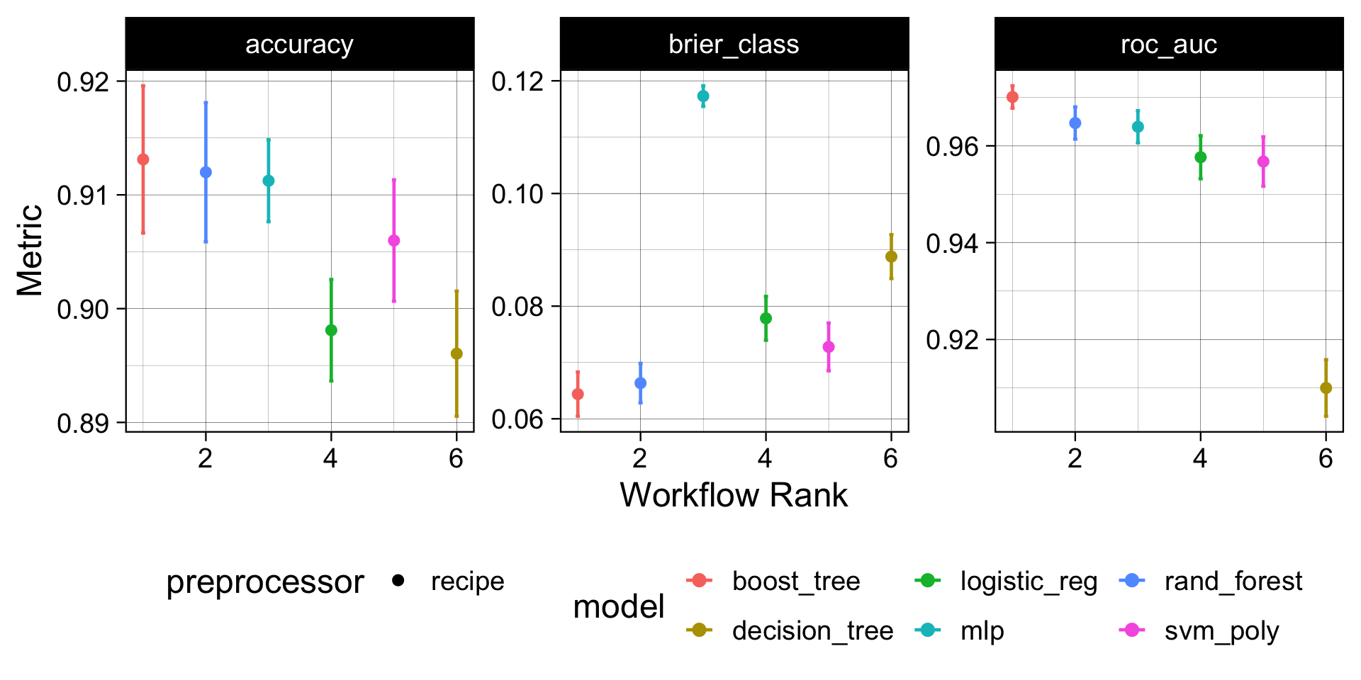
How to read this plot: Each dot is the mean CV metric across 10 folds; whiskers are ±1 SE. A model whose interval is highest and tightest is both accurate and consistent. Overlapping intervals mean the difference may not be meaningful — prefer the simpler model when in doubt.

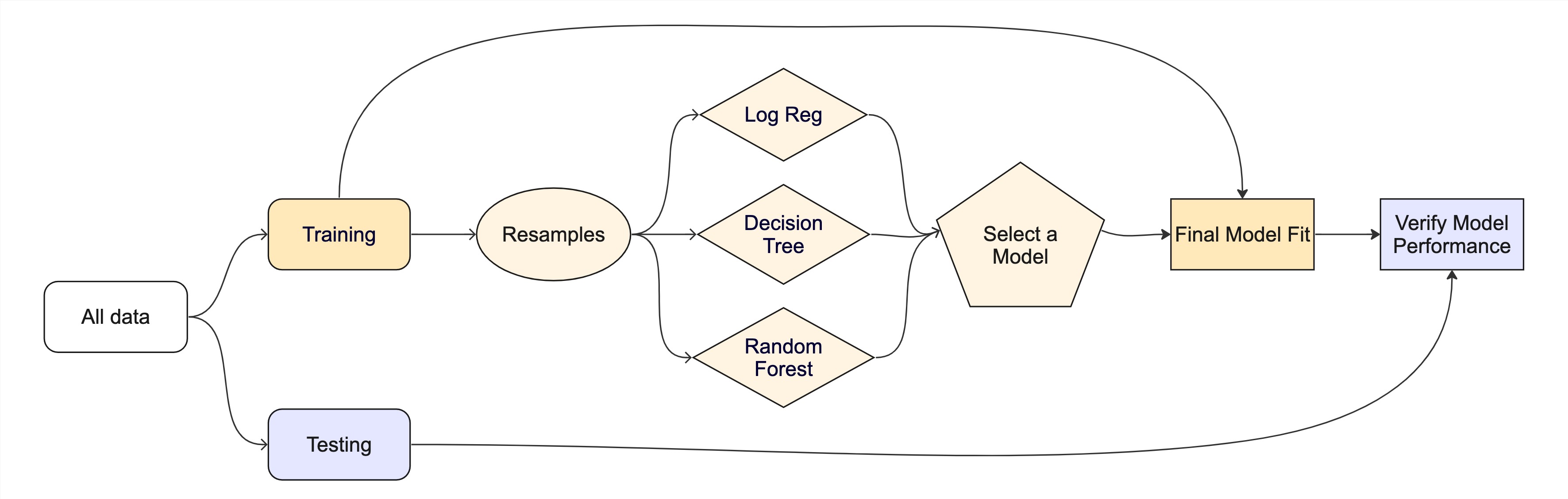
Model Evaluation

Since the boosted-tree model gave the best out-of-the-box performance, we can:

Select that model specification.
Refit it to the full training set (no more cross-validation needed here — we’ve already used the folds to make the comparison).
Assess it once against the held-out forested_test set to get an honest estimate of skill on unseen data.

final_fit <- workflow() |>
  add_recipe(forested_recipe) |>
  # Selected model
  add_model(b_model) |>
  # Trained on the full training dataset
  fit(data = forested_train) |>
  # Validated against held-out data
  augment(new_data = forested_test)

# Final results
metrics(final_fit,  truth = forested, estimate = .pred_class)
#> # A tibble: 2 × 3
#>   .metric  .estimator .estimate
#>   <chr>    <chr>          <dbl>
#> 1 accuracy binary         0.909
#> 2 kap      binary         0.817
conf_mat(final_fit, truth = forested, estimate = .pred_class)
#>           Truth
#> Prediction Yes  No
#>        Yes 911  98
#>        No   63 706

Important

This is the untuned boosted tree — the same model we compared with workflow_set() above. It’s a baseline. In the tuning section below we’ll search over trees, learn_rate, and min_n for this same model and fit the final tuned version with last_fit() against this same forested_split. Expect the tuned version to beat this number.

The whole game - status update

Recapping

library(tidymodels)
library(forested)

# Set a seed
set.seed(123)

# Initialize split
forested_split <- initial_split(forested, strata = forested)
forested_train <- training(forested_split)
forested_test  <- testing(forested_split)

# Build Resamples
forested_folds <- vfold_cv(forested_train, v = 10)

# Winning model from the model zoo comparison
b_mod_eval <- boost_tree(
  trees = 15, tree_depth = 6, learn_rate = 0.3, loss_reduction = 0, mtry = 1
) |>
  set_engine("xgboost") |>
  set_mode("classification")

# Workflow using the recipe built earlier
forested_wflow <- workflow(forested_recipe, b_mod_eval)
forested_fit   <- fit(forested_wflow, forested_train)

# Extracting Predictions:
augment(forested_fit, new_data = forested_train)
#> # A tibble: 5,329 × 22
#>    .pred_class .pred_Yes .pred_No forested  year elevation eastness northness
#>    <fct>           <dbl>    <dbl> <fct>    <dbl>     <dbl>    <dbl>     <dbl>
#>  1 Yes           0.798      0.202 No        2005       164      -84        53
#>  2 No            0.393      0.607 No        2005      1713      -66        75
#>  3 No            0.0235     0.977 No        2014       542      -32       -94
#>  4 No            0.0464     0.954 No        2014       759       -2       -99
#>  5 No            0.00827    0.992 No        2014       119        0         0
#>  6 No            0.0456     0.954 No        2014       246       22       -97
#>  7 No            0.0137     0.986 No        2014       235        0      -100
#>  8 No            0.00859    0.991 No        2014       324       71        70
#>  9 No            0.0106     0.989 No        2014       419       86       -49
#> 10 No            0.00792    0.992 No        2014       308      -70       -70
#> # ℹ 5,319 more rows
#> # ℹ 14 more variables: roughness <dbl>, tree_no_tree <fct>, dew_temp <dbl>,
#> #   precip_annual <dbl>, temp_annual_mean <dbl>, temp_annual_min <dbl>,
#> #   temp_annual_max <dbl>, temp_january_min <dbl>, vapor_min <dbl>,
#> #   vapor_max <dbl>, canopy_cover <dbl>, lon <dbl>, lat <dbl>, land_type <fct>

Evaluation

So far we have used metrics and collect_metrics to evaluate and compare models
The default metrics for classification problems are: accuracy, brier_class, roc_auc
- All classification metrics stem from the classic confusion matrix

The default metrics for regression problems are: rsq, rmse, mae
- The majority of these are measures of correlation and residual error

Classification:

Training-set metrics are optimistic

The next examples evaluate against forested_train — the same data the model saw during fitting.

These numbers look good by design: the model has already seen this data.
For an honest estimate of performance on new data, always use cross-validation results (collect_metrics() on resamples) or the held-out forested_test via last_fit().

We use training data here only to illustrate what each metric measures with clean, consistent outputs.

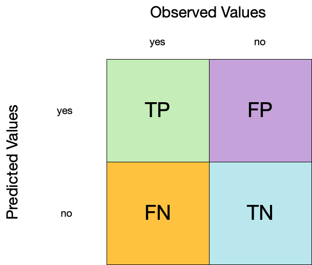
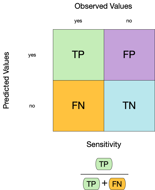
Confusion matrix

A confusion matrix is a table that describes the performance of a classification model on a set of data for which the true values are known.
It counts the number of accurate and false predictions, separated by the truth state

augment(forested_fit, new_data = forested_train) |>
  conf_mat(truth = forested, estimate = .pred_class)
#>           Truth
#> Prediction  Yes   No
#>        Yes 2779  202
#>        No   141 2207

What to do with a confusion matrix

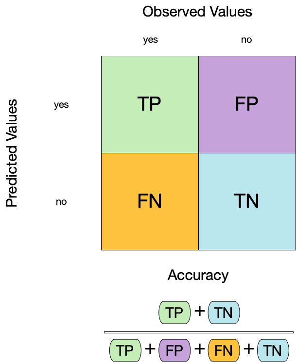
1. Accuracy

Accuracy is the proportion of true results (both true positives and true negatives) among the total number of cases examined.
It is a measure of the correctness of the model’s predictions.
It is the most common metric used to evaluate classification models.

augment(forested_fit, new_data = forested_train) |>
  accuracy(truth = forested, estimate = .pred_class)
#> # A tibble: 1 × 3
#>   .metric  .estimator .estimate
#>   <chr>    <chr>          <dbl>
#> 1 accuracy binary         0.936

2. Sensitivity

Sensitivity is the proportion of true positives to the sum of true positives and false negatives.
It is useful for identifying the presence of a condition.
It is also known as the true positive rate, recall, or probability of detection.

augment(forested_fit, new_data = forested_train) |>
  sensitivity(truth = forested, estimate = .pred_class)
#> # A tibble: 1 × 3
#>   .metric     .estimator .estimate
#>   <chr>       <chr>          <dbl>
#> 1 sensitivity binary         0.952

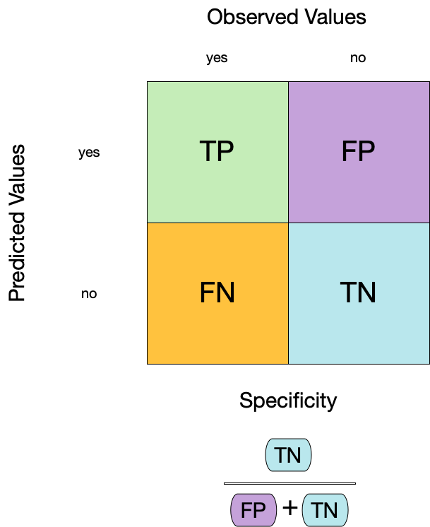
3. Specificity

Specificity is the proportion of true negatives to the sum of true negatives and false positives.
It is useful for identifying the absence of a condition.
It is also known as the true negative rate, and is the complement of sensitivity.

augment(forested_fit, new_data = forested_train) |>
  sensitivity(truth = forested, estimate = .pred_class)
#> # A tibble: 1 × 3
#>   .metric     .estimator .estimate
#>   <chr>       <chr>          <dbl>
#> 1 sensitivity binary         0.952

augment(forested_fit, new_data = forested_train) |>
  specificity(truth = forested, estimate = .pred_class)
#> # A tibble: 1 × 3
#>   .metric     .estimator .estimate
#>   <chr>       <chr>          <dbl>
#> 1 specificity binary         0.916

Two class data

These metrics assume that we know the threshold for converting “soft” probability predictions into “hard” class predictions.

For example, if the predicted probability of a tree is 0.7, we might say that the model predicts “Tree” for that observation.
If the predicted probability of a tree is 0.4, we might say that the model predicts “No tree” for that observation.
The threshold is the value that separates the two classes.
The default threshold is 0.5, but this can be changed.

Is a 50% threshold good?

What happens if we say that we need to be 80% sure to declare an event?

sensitivity ⬇️, specificity ⬆️

What happens for a 20% threshold?

sensitivity ⬆️, specificity ⬇️

Environmental context: For rare or high-stakes events — flood detection, wildfire risk, species presence — a false negative (missing a real event) is usually far more costly than a false positive. This pushes the threshold lower to maximize sensitivity, accepting more false alarms. The right threshold is a domain decision, not a statistical one.

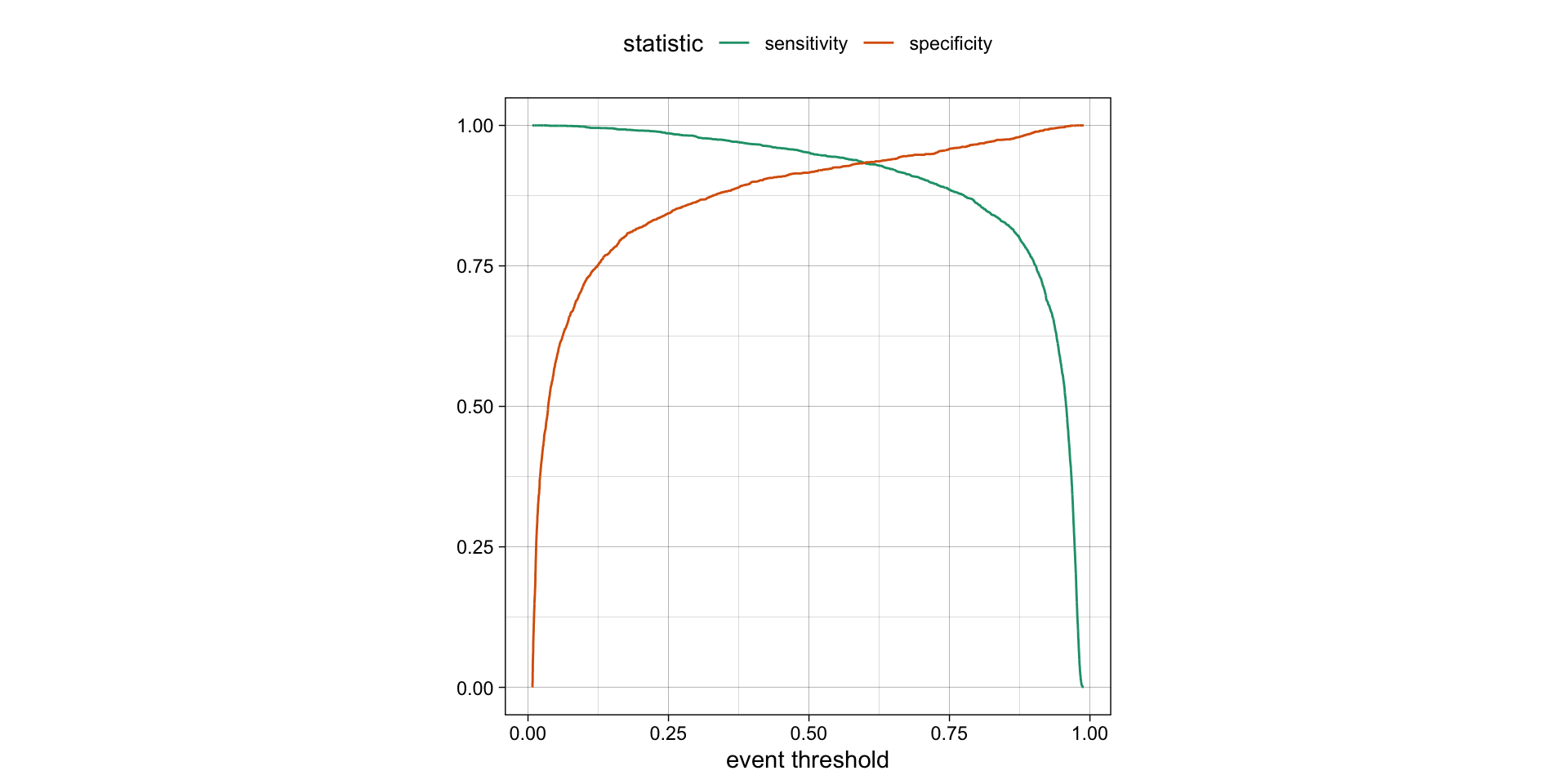
Varying the threshold

The threshold can be varied to see how it affects the sensitivity and specificity of the model.
This is done by plotting the sensitivity and specificity against the threshold.
The threshold is varied from 0 to 1, and the sensitivity and specificity are calculated at each threshold.
The plot shows the trade-off between sensitivity and specificity at different thresholds.
The threshold can be chosen based on the desired balance between sensitivity and specificity.

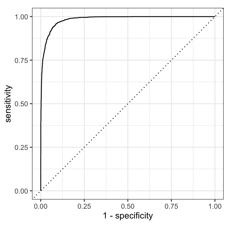
ROC curves

The previous plot showed sensitivity and specificity each varying with threshold. An ROC curve shows the same tradeoff differently: sweep every possible threshold and plot

false positive rate (1 − specificity) on the x-axis
true positive rate (sensitivity) on the y-axis

The diagonal line = random guessing (AUC 0.5). A good model hugs the top-left corner.

ROC curves

ROC AUC = area under the ROC curve = the model’s ability to separate the two classes.

Intuition: give the model a random forested and a random non-forested hexagon — AUC is the probability it scores the forested one higher.

ROC AUC = 1 💯 — perfect separation
ROC AUC = 0.5 😐 — no better than flipping a coin (the diagonal)
ROC AUC < 0.5 😱 — actively worse than random

ROC curves

roc_curve() returns a tibble with one row per evaluated threshold — sensitivity and specificity at each point. roc_auc() summarises the whole curve into one number.

(AUC 0.7–0.8 = acceptable, 0.8–0.9 = good, >0.9 = excellent)

# Assumes _first_ factor level is event; there are options to change that
augment(forested_fit, new_data = forested_train) |>
  roc_curve(truth = forested, .pred_Yes) |>
  dplyr::slice(1, 20, 50)   # peek at 3 rows from the threshold sweep

#> # A tibble: 3 × 3
#>   .threshold specificity sensitivity
#>        <dbl>       <dbl>       <dbl>
#> 1 -Inf            0                1
#> 2    0.00869      0.0477           1
#> 3    0.00960      0.0863           1

augment(forested_fit, new_data = forested_train) |>
  roc_auc(truth = forested, .pred_Yes)

#> # A tibble: 1 × 3
#>   .metric .estimator .estimate
#>   <chr>   <chr>          <dbl>
#> 1 roc_auc binary         0.984

Brier score

The Brier score is a measure of how well the predicted probabilities of an event match the actual outcomes.
It is the mean squared difference between predicted probabilities and actual outcomes.
The Brier score is a number between 0 and 1.
The Brier score is analogous to the mean squared error in regression models:
Brier = 1 😱
- predicted probabilities are completely wrong
Brier = 0.5 😐
- bad
Brier < 0.25
- acceptable
Brier = 0 💯
- predicted probabilities are perfect

\[ Brier_{class} = \frac{1}{N}\sum_{i=1}^N\sum_{k=1}^C (y_{ik} - \hat{p}_{ik})^2 \]

Brier score

augment(forested_fit, new_data = forested_train) |>  
  brier_class(truth = forested, .pred_Yes) 
#> # A tibble: 1 × 3
#>   .metric     .estimator .estimate
#>   <chr>       <chr>          <dbl>
#> 1 brier_class binary        0.0480

Separation vs calibration

The ROC captures separation. - The ROC curve shows the trade-off between sensitivity and specificity at different thresholds.

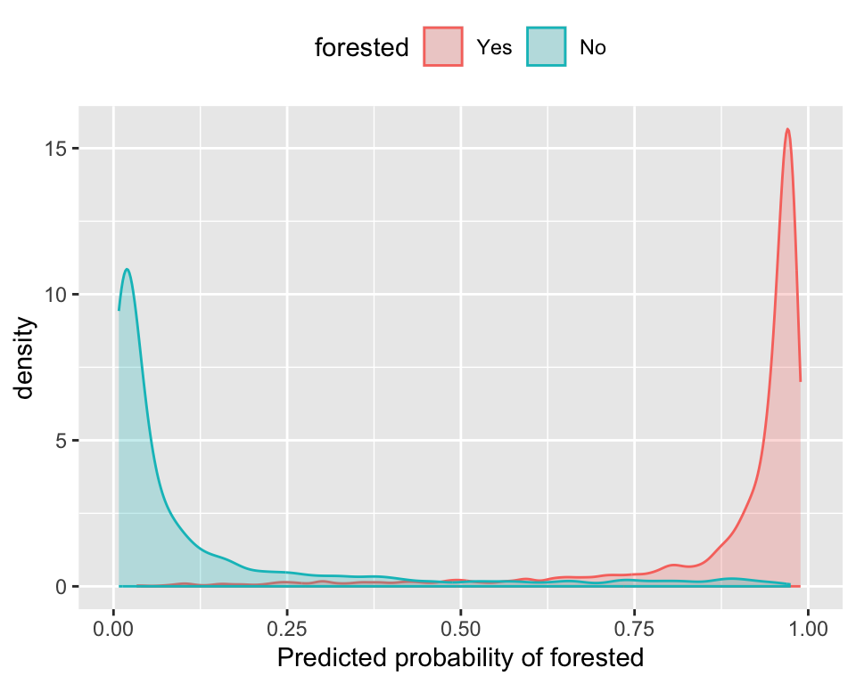
The Brier score captures calibration. - The Brier score is a measure of how well the predicted probabilities of an event match the actual outcomes.

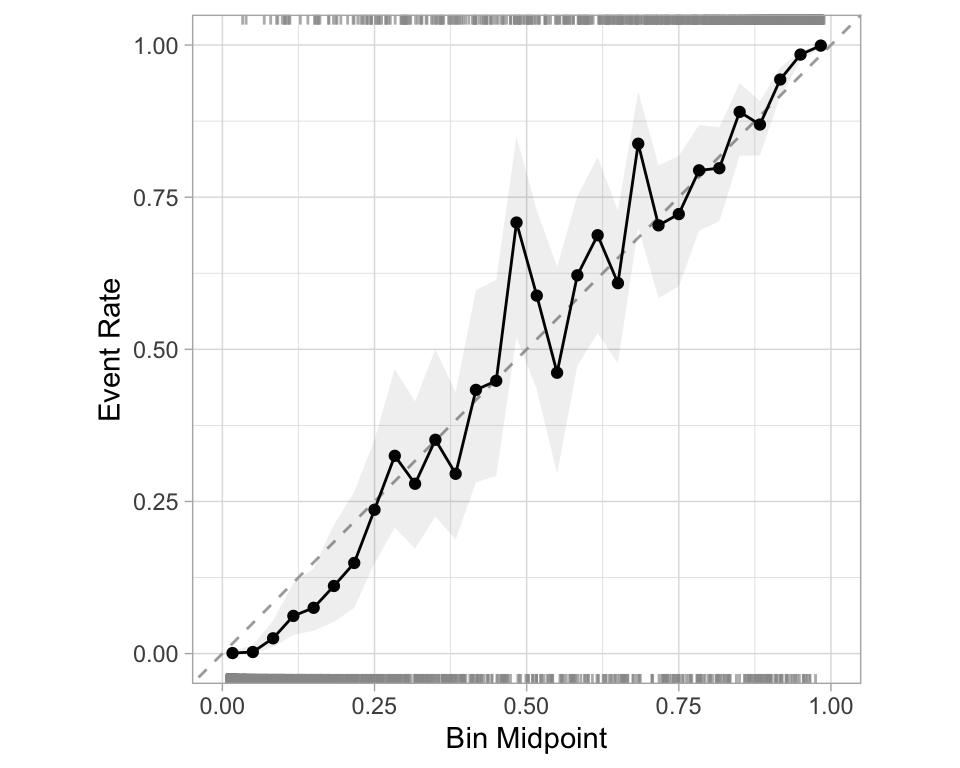
Good separation: the densities don’t overlap.
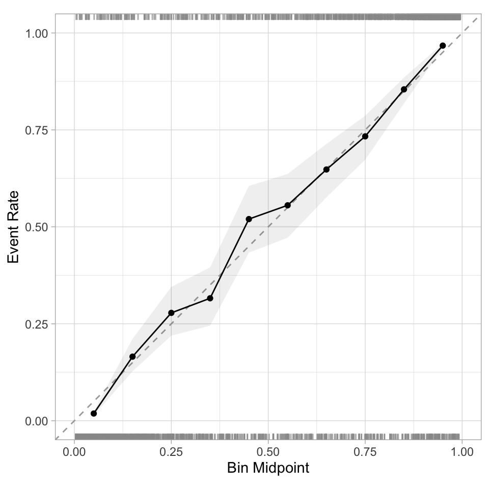
Good calibration: the calibration line follows the diagonal.

Calibration plot: We bin observations according to predicted probability. In the bin for 20%-30% predicted prob, we should see an event rate of ~25% if the model is well-calibrated.

Regression

R-squared (\(R^2\))

Measures how well the model explains the variance in the data.
Formula:

\[ R^2 = 1 - \frac{SS_{res}}{SS_{tot}} \] where:
- \(SS_{res}\) is the sum of squared residuals.

\(SS_{tot}\) is the total sum of squares.
Values range from \(-\infty\) to 1.
- 1: Perfect fit
- 0: No improvement over mean prediction
- Negative: Worse than just using the mean

Root Mean Squared Error (RMSE)

Measures the model’s prediction error in the same unit as the dependent variable.
Formula:

\[ RMSE = \sqrt{\frac{1}{n} \sum_{i=1}^{n} (y_i - \hat{y}_i)^2} \]

where: - \(y_i\) is the actual value. - \(\hat{y}_i\) is the predicted value.

Penalizes large errors more than MAE.
Lower RMSE indicates better model performance.

Mean Absolute Error (MAE)

Measures average absolute errors between predictions and actual values.
Formula:

\[ MAE = \frac{1}{n} \sum_{i=1}^{n} |y_i - \hat{y}_i| \]

Less sensitive to outliers than RMSE.
Lower MAE indicates better model performance.

Comparing Metrics

Metric	Interpretation	Sensitivity to Outliers
\(R^2\)	Variance explained	Moderate
RMSE	Penalizes large errors more	High
MAE	Average error size	Low

Choosing the Right Metric

Use \(R^2\) to assess model fit and explainability.
Use RMSE if large errors are especially undesirable.
Use MAE for a more interpretable, robust metric.

Custom Metric Sets

We can use metric_set() to combine multiple calculations into one

forested_metrics <- metric_set(accuracy, specificity, sensitivity)

augment(forested_fit, new_data = forested_train) |>
  forested_metrics(truth = forested, estimate = .pred_class)
#> # A tibble: 3 × 3
#>   .metric     .estimator .estimate
#>   <chr>       <chr>          <dbl>
#> 1 accuracy    binary         0.936
#> 2 specificity binary         0.916
#> 3 sensitivity binary         0.952

Metrics and metric sets work with grouped data frames!

augment(forested_fit, new_data = forested_train) |>
  group_by(tree_no_tree) |>
  accuracy(truth = forested, estimate = .pred_class)
#> # A tibble: 2 × 4
#>   tree_no_tree .metric  .estimator .estimate
#>   <fct>        <chr>    <chr>          <dbl>
#> 1 Tree         accuracy binary         0.942
#> 2 No tree      accuracy binary         0.928

augment(forested_fit, new_data = forested_train) |>
  group_by(tree_no_tree) |>
  specificity(truth = forested, estimate = .pred_class)
#> # A tibble: 2 × 4
#>   tree_no_tree .metric     .estimator .estimate
#>   <fct>        <chr>       <chr>          <dbl>
#> 1 Tree         specificity binary         0.428
#> 2 No tree      specificity binary         0.976

Note

The specificity for "Tree" is a good bit lower than it is for "No tree".

Among hexagons where the remote sensing index shows tree cover, the model more often predicts forested even when the ground truth is non-forested — these are the plots most likely to be confused.

Recap — where we are

Reusing what we already built

We’re going to keep tuning on the same forested classification problem — no new data, no new recipe — so the story stays coherent.

From earlier in this deck we already have:

forested_split — 75/25 stratified split
forested_train, forested_test — 75% training, 25% test
forested_folds — 10-fold CV on the training set
forested_recipe — impute → dummy → normalize

forested_recipe

Optimizing Models via Hyperparameter Tuning

Tuning parameters

Some model or preprocessing parameters cannot be estimated directly from the data.
Try different values and measure their performance.

Find good values for these parameters.

Once the value(s) of the parameter(s) are determined, a model can be finalized by fitting the model to the entire training set.

Tagging parameters for tuning

With tidymodels, you can mark the parameters that you want to optimize with a value of tune().

The function itself just returns… itself:

tune()

#> tune()

str(tune())

#>  language tune()

# optionally add a label
tune("Marker")

#> tune("Marker")

Boosted Trees

Earlier today, the boosted tree was our best untuned model — let’s see how much further we can push it with tuning.

Boosted Trees are popular ensemble methods that build a sequence of tree models.

Each tree uses the results of the previous tree to better predict samples, especially those that have been poorly predicted.

Each tree in the ensemble is saved and new samples are predicted using a weighted average of the votes of each tree in the ensemble.

Boosted Tree Tuning Parameters

Some possible parameters:

mtry: The number of predictors randomly sampled at each split (in \([1, ncol(x)]\) or \((0, 1]\)).
trees: The number of trees (\([1, \infty]\), but usually up to thousands)
min_n: The number of samples needed to further split (\([1, n]\)).
learn_rate: The rate that each tree adapts from previous iterations (\((0, \infty]\), usual maximum is 0.1).
stop_iter: The number of iterations of boosting where no improvement was shown before stopping (\([1, trees]\))

Boosted Tree Tuning Parameters

b_mod <-
  boost_tree(trees = tune(), learn_rate = tune()) |>
  set_mode("classification") |>
  set_engine("xgboost")

(b_wflow <- workflow(forested_recipe, b_mod))

#> ══ Workflow ════════════════════════════════════════════════════════════════════════════════════════════════════════════════════════════════════════════════════════════════════════════════════════════
#> Preprocessor: Recipe
#> Model: boost_tree()
#> 
#> ── Preprocessor ────────────────────────────────────────────────────────────────────────────────────────────────────────────────────────────────────────────────────────────────────────────────────────
#> 3 Recipe Steps
#> 
#> • step_impute_mean()
#> • step_dummy()
#> • step_normalize()
#> 
#> ── Model ───────────────────────────────────────────────────────────────────────────────────────────────────────────────────────────────────────────────────────────────────────────────────────────────
#> Boosted Tree Model Specification (classification)
#> 
#> Main Arguments:
#>   trees = tune()
#>   learn_rate = tune()
#> 
#> Computational engine: xgboost

Optimize tuning parameters

The main two strategies for optimization are:

Grid search 💠 which tests a pre-defined set of candidate values
Iterative search 🌀 which suggests/estimates new values of candidate parameters to evaluate

1. Grid search

Most basic (but very effective) way to tune models
A small grid of points trying to minimize the error via learning rate:

1. Grid search

In reality we would probably sample the space more densely:

2. Iterative Search

We could start with a few points and search the space:

Grid Search Example

Parameters

The tidymodels framework provides pre-defined information on tuning parameters (such as their type, range, transformations, etc).
The extract_parameter_set_dials() function extracts these tuning parameters and the info.

Grids

Create your grid manually or automatically.
The grid_*() functions can make a grid.

Different types of grids

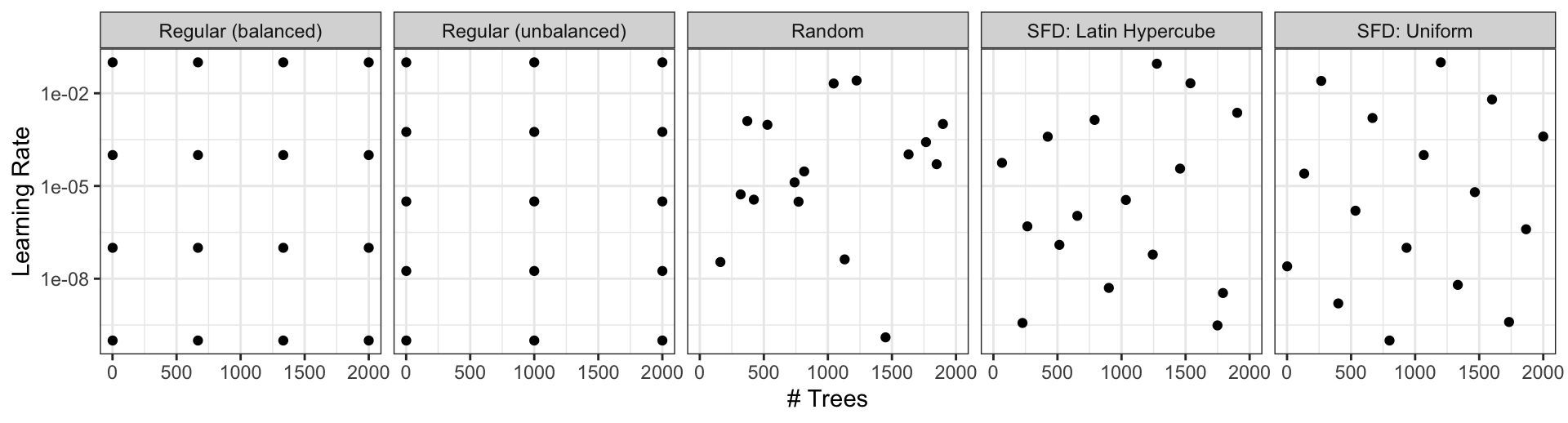
Space-filling designs (SFD) attempt to cover the parameter space without redundant candidates. We recommend these the most.

Create a grid

# Extract
(b_wflow |>
  extract_parameter_set_dials())

# Individual functions:
(trees())
(learn_rate())

A parameter set can be updated (e.g. to change the ranges).

Create a grid

The grid_*() functions create a grid of parameter values to evaluate.
The grid_space_filling() function creates a space-filling design (SFD) of parameter values to evaluate.
The grid_regular() function creates a regular grid of parameter values to evaluate.
The grid_random() function creates a random grid of parameter values to evaluate.
The grid_latin_hypercube() function creates a Latin hypercube design of parameter values to evaluate.
The grid_max_entropy() function creates a maximum entropy design of parameter values to evaluate.

Create a SFD curve

set.seed(12)

(grid <-
  b_wflow |>
  extract_parameter_set_dials() |>
  grid_space_filling(size = 25))

#> # A tibble: 25 × 2
#>    trees learn_rate
#>    <int>      <dbl>
#>  1     1    0.0287 
#>  2    84    0.00536
#>  3   167    0.121  
#>  4   250    0.00162
#>  5   334    0.0140 
#>  6   417    0.0464 
#>  7   500    0.196  
#>  8   584    0.00422
#>  9   667    0.00127
#> 10   750    0.0178 
#> # ℹ 15 more rows

Create a regular grid

set.seed(12)

(grid <-
  b_wflow |>
  extract_parameter_set_dials() |>
  grid_regular(levels = 4))

#> # A tibble: 16 × 2
#>    trees learn_rate
#>    <int>      <dbl>
#>  1     1    0.001  
#>  2   667    0.001  
#>  3  1333    0.001  
#>  4  2000    0.001  
#>  5     1    0.00681
#>  6   667    0.00681
#>  7  1333    0.00681
#>  8  2000    0.00681
#>  9     1    0.0464 
#> 10   667    0.0464 
#> 11  1333    0.0464 
#> 12  2000    0.0464 
#> 13     1    0.316  
#> 14   667    0.316  
#> 15  1333    0.316  
#> 16  2000    0.316

Update parameter ranges

b_param <- 
  b_wflow |> 
  extract_parameter_set_dials() |> 
  update(trees = trees(c(1L, 100L)),
         learn_rate = learn_rate(c(-5, -1)))

set.seed(712)
(grid <- 
  b_param |> 
  grid_space_filling(size = 25))

#> # A tibble: 25 × 2
#>    trees learn_rate
#>    <int>      <dbl>
#>  1     1  0.00215  
#>  2     5  0.000147 
#>  3     9  0.0215   
#>  4    13  0.0000215
#>  5    17  0.000681 
#>  6    21  0.00464  
#>  7    25  0.0464   
#>  8    29  0.0001   
#>  9    34  0.0000147
#> 10    38  0.001    
#> # ℹ 15 more rows

The results

grid |> 
  ggplot(aes(trees, learn_rate)) +
  geom_point(size = 4) +
  scale_y_log10()

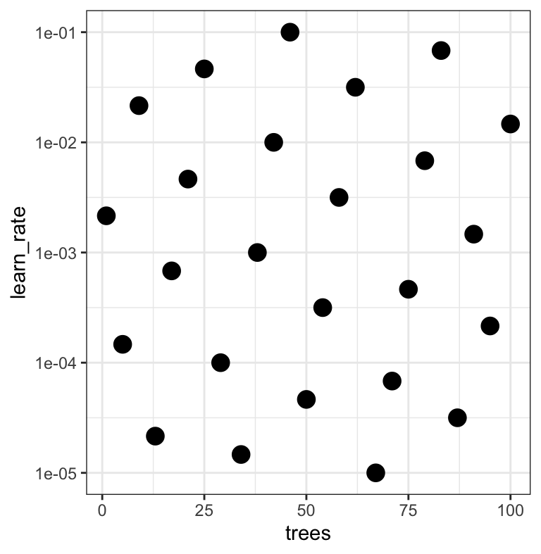
Note that the learning rates are uniform on the log-10 scale — both tuning parameters are shown.

Use the `tune_*()` functions to tune models

Choosing tuning parameters

Let’s take our previous model and tune more parameters:

b_mod <-
  boost_tree(trees = tune(), learn_rate = tune(), min_n = tune()) |>
  set_mode("classification") |>
  set_engine("xgboost")

b_wflow <- workflow(forested_recipe, b_mod)

# Widen the trees range for the search
b_param <-
  b_wflow |>
  extract_parameter_set_dials() |>
  update(trees = trees(c(1L, 1000L)))

Grid Search

set.seed(9)
ctrl <- control_grid(save_pred = TRUE)

b_res <-
  b_wflow |>
  tune_grid(
    resamples = forested_folds,
    grid = 25,
    # The options below are not required by default
    param_info = b_param,
    control = ctrl,
    metrics = metric_set(roc_auc, accuracy, brier_class)
  )

Grid Search

b_res

#> # Tuning results
#> # 10-fold cross-validation 
#> # A tibble: 10 × 5
#>    splits             id     .metrics          .notes           .predictions         
#>    <list>             <chr>  <list>            <list>           <list>               
#>  1 <split [5116/569]> Fold01 <tibble [75 × 7]> <tibble [0 × 4]> <tibble [14,225 × 9]>
#>  2 <split [5116/569]> Fold02 <tibble [75 × 7]> <tibble [0 × 4]> <tibble [14,225 × 9]>
#>  3 <split [5116/569]> Fold03 <tibble [75 × 7]> <tibble [0 × 4]> <tibble [14,225 × 9]>
#>  4 <split [5116/569]> Fold04 <tibble [75 × 7]> <tibble [0 × 4]> <tibble [14,225 × 9]>
#>  5 <split [5116/569]> Fold05 <tibble [75 × 7]> <tibble [0 × 4]> <tibble [14,225 × 9]>
#>  6 <split [5117/568]> Fold06 <tibble [75 × 7]> <tibble [0 × 4]> <tibble [14,200 × 9]>
#>  7 <split [5117/568]> Fold07 <tibble [75 × 7]> <tibble [0 × 4]> <tibble [14,200 × 9]>
#>  8 <split [5117/568]> Fold08 <tibble [75 × 7]> <tibble [0 × 4]> <tibble [14,200 × 9]>
#>  9 <split [5117/568]> Fold09 <tibble [75 × 7]> <tibble [0 × 4]> <tibble [14,200 × 9]>
#> 10 <split [5117/568]> Fold10 <tibble [75 × 7]> <tibble [0 × 4]> <tibble [14,200 × 9]>

Grid results

autoplot(b_res)

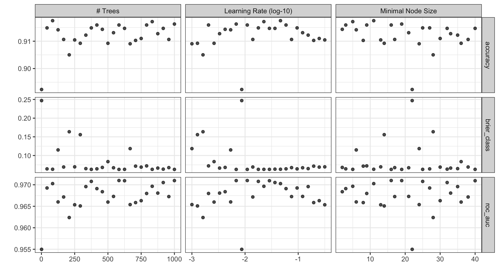
Tuning results

collect_metrics(b_res)

#> # A tibble: 75 × 9
#>    trees min_n learn_rate .metric     .estimator   mean     n   std_err .config         
#>    <int> <int>      <dbl> <chr>       <chr>       <dbl> <int>     <dbl> <chr>           
#>  1     1    22    0.00866 accuracy    binary     0.892     10 0.00365   pre0_mod01_post0
#>  2     1    22    0.00866 brier_class binary     0.247     10 0.0000270 pre0_mod01_post0
#>  3     1    22    0.00866 roc_auc     binary     0.955     10 0.00284   pre0_mod01_post0
#>  4    42    27    0.0953  accuracy    binary     0.915     10 0.00365   pre0_mod02_post0
#>  5    42    27    0.0953  brier_class binary     0.0642    10 0.00220   pre0_mod02_post0
#>  6    42    27    0.0953  roc_auc     binary     0.969     10 0.00229   pre0_mod02_post0
#>  7    84    11    0.0464  accuracy    binary     0.918     10 0.00248   pre0_mod03_post0
#>  8    84    11    0.0464  brier_class binary     0.0632    10 0.00206   pre0_mod03_post0
#>  9    84    11    0.0464  roc_auc     binary     0.970     10 0.00207   pre0_mod03_post0
#> 10   125     6    0.00536 accuracy    binary     0.914     10 0.00382   pre0_mod04_post0
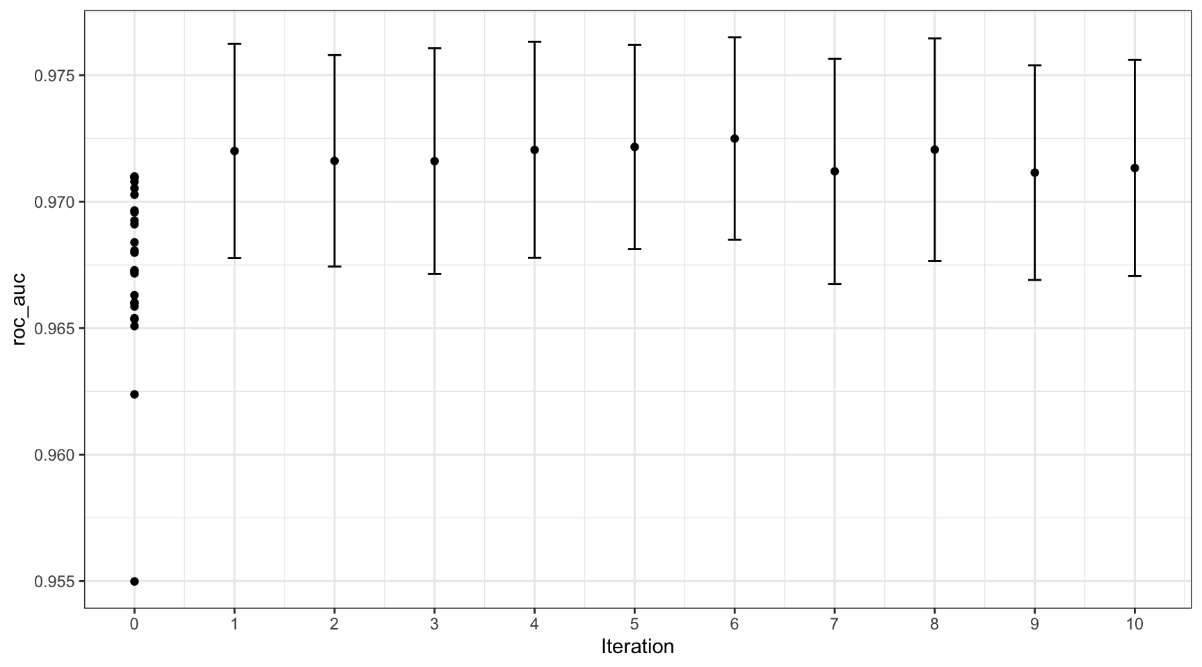
#> # ℹ 65 more rows

Iterative Search — Bayesian Optimization

Fits a Gaussian process surrogate model on results so far
Suggests the most promising next candidate (balances exploration vs. exploitation)
Requires far fewer iterations than grid search to reach similar quality
Can warm-start from an existing grid search result to avoid re-evaluating already-known points

Key function: tune_bayes() — same syntax as tune_grid()

Bayesian Search Example

set.seed(9)
b_bayes <-
  b_wflow |>
  tune_bayes(
    resamples  = forested_folds,
    initial    = b_res,       # warm-start: skip candidates already evaluated
    iter       = 10,
    param_info = b_param,
    metrics    = metric_set(roc_auc)
  )

show_best(b_bayes, metric = "roc_auc")

#> # A tibble: 5 × 10
#>   trees min_n learn_rate .metric .estimator  mean     n std_err .config .iter
#>   <int> <int>      <dbl> <chr>   <chr>      <dbl> <int>   <dbl> <chr>   <int>
#> 1   344     5     0.0217 roc_auc binary     0.972    10 0.00180 iter06      6
#> 2   229     2     0.0237 roc_auc binary     0.972    10 0.00181 iter05      5
#> 3   982    25     0.0155 roc_auc binary     0.972    10 0.00197 iter08      8
#> 4   404    15     0.0290 roc_auc binary     0.972    10 0.00192 iter04      4
#> 5   569    25     0.0247 roc_auc binary     0.972    10 0.00190 iter01      1

Tip

Passing initial = b_res means Bayesian search starts from what the grid search already learned — no wasted evaluations on territory already explored.

Bayesian Search Results

autoplot(b_bayes, type = "performance")

Grid Search vs Bayesian Optimization

	Grid Search	Bayesian Optimization
How it works	Pre-defined candidates evaluated in parallel	Learns from previous results, suggests next point
Best when	Compute is cheap; reproducibility matters	Fitting is expensive; budget is tight
Parallelism	Fully parallel	Sequential by design
Warm starting	No	Yes — can reuse grid results with `initial = b_res`
tidymodels fn	`tune_grid()`	`tune_bayes()`

In practice: start with a grid search to understand the landscape, then hand the results to Bayesian search for refinement.

Choose a parameter combination

show_best(b_res, metric = "roc_auc")

#> # A tibble: 5 × 9
#>   trees min_n learn_rate .metric .estimator  mean     n std_err .config         
#>   <int> <int>      <dbl> <chr>   <chr>      <dbl> <int>   <dbl> <chr>           
#> 1   583    16    0.0110  roc_auc binary     0.971    10 0.00197 pre0_mod15_post0
#> 2  1000    19    0.00681 roc_auc binary     0.971    10 0.00204 pre0_mod25_post0
#> 3   625    40    0.0287  roc_auc binary     0.971    10 0.00199 pre0_mod16_post0
#> 4   375    25    0.0178  roc_auc binary     0.971    10 0.00213 pre0_mod10_post0
#> 5   916    32    0.0365  roc_auc binary     0.971    10 0.00203 pre0_mod23_post0

Choose a parameter combination

Create your own tibble for final parameters or use one of the tune::select_*() functions:

(b_best <- select_best(b_res, metric = "roc_auc"))

#> # A tibble: 1 × 4
#>   trees min_n learn_rate .config         
#>   <int> <int>      <dbl> <chr>           
#> 1   583    16     0.0110 pre0_mod15_post0

Checking Calibration

library(probably)

b_res |>
  collect_predictions(
    parameters = b_best
  ) |>
  cal_plot_breaks(
    truth = forested,
    estimate = .pred_Yes,
    num_breaks = 10
  )

The final fit!

Suppose that we are happy with our model.

Let’s fit the model on the training set and verify our performance using the test set.

last_fit(workflow, split) does three things in one call:

Fits the finalized workflow on the full training set
Predicts on the held-out test set
Returns metrics and predictions — ready for collect_metrics() / collect_predictions()

Call last_fit() once, at the very end. Using the test set to make any modeling decisions (threshold, features, model choice) invalidates it as an honest estimate.

# the boosted tree workflow can be `finalized` with the best parameters
final_workflow <- finalize_workflow(b_wflow, b_best)

# forested_split carries train + test — last_fit() fits on train, evaluates on test
(final_fit <- last_fit(final_workflow, forested_split))

#> # Resampling results
#> # Manual resampling 
#> # A tibble: 1 × 6
#>   splits              id               .metrics         .notes           .predictions         .workflow 
#>   <list>              <chr>            <list>           <list>           <list>               <list>    
#> 1 <split [5329/1778]> train/test split <tibble [3 × 4]> <tibble [0 × 4]> <tibble [1,778 × 6]> <workflow>

The final fit!

# Metrics on the held-out test set
collect_metrics(final_fit)

#> # A tibble: 3 × 4
#>   .metric     .estimator .estimate .config        
#>   <chr>       <chr>          <dbl> <chr>          
#> 1 accuracy    binary        0.908  pre0_mod0_post0
#> 2 roc_auc     binary        0.968  pre0_mod0_post0
#> 3 brier_class binary        0.0666 pre0_mod0_post0

# Confusion matrix on the held-out test set
collect_predictions(final_fit) |>
  conf_mat(truth = forested, estimate = .pred_class)

#>           Truth
#> Prediction Yes  No
#>        Yes 910 100
#>        No   64 704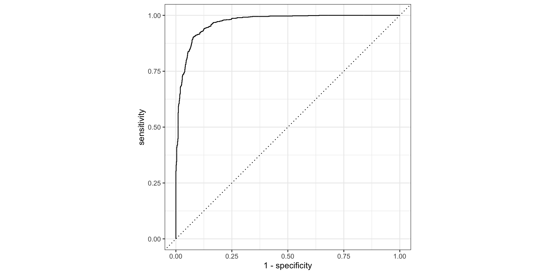

# ROC curve on the held-out test set
collect_predictions(final_fit) |>
  roc_curve(truth = forested, .pred_Yes) |>
  autoplot()

What did the model learn?

library(vip)

extract_fit_parsnip(final_fit) |>
  vip(num_features = 15, geom = "col") +
  labs(title = "Boosted tree: top predictors of forested status") +
  theme_linedraw(14)

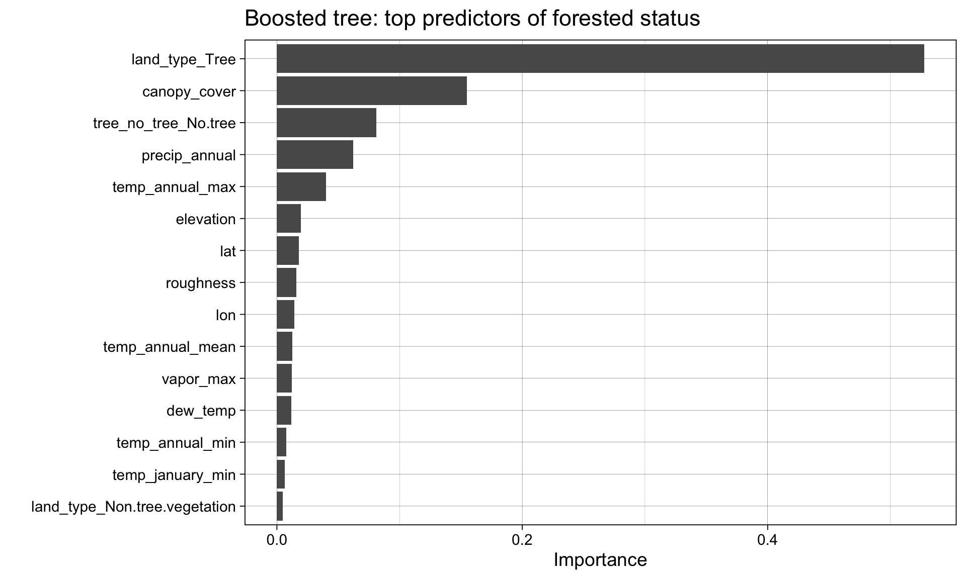
Variable importance connects performance back to science: which features drove the prediction?

Note

Recall from week 5: different families give different importance estimates — logistic regression uses standardized coefficients, random forest uses impurity reduction, boosted trees use gain.

Agreement across families = robust signal. Disagreement = worth investigating.

Week 6

Introduction

By the end of today you will be able to…

Classification vs. Regression

Classification Models

Examples:

Common Algorithms:

Regression Models

Examples:

Common Algorithms:

Choosing the Right Model

Model Selection Considerations

Load Required Libraries

Data Preparation

Machine Learning Specifications in tidymodels

Unified Interface for ML Models

Metric vocabulary — what collect_metrics() will show us

What are hyperparameters?

Today’s model zoo, at a glance

Linear Regression

Components of Linear Regression

Linear Regression in tidymodels

Specification

engines & modes

Example

Logistic Regression

Components of Logistic Regression

Variants of Logistic Regression

Building a Logistic Regression Model

Constructing a Logistic Regression Model involves:

Hyperparameters in Logistic Regression

Logistic Regression in tidymodels

Specification

engines & modes

Example

Decision Tree

Components of a Decision Tree

Building a Decision Tree

Constructing a Decision Tree involves:

Splitting Criteria

Hyperparameters in Decision Trees

Decision Tree using tidymodels

Specification

engines & modes

Example

Random Forest

Components of a Random Forest

Building a Random Forest

Constructing a Random Forest involves:

Hyperparameters in Random Forest

Random Forest Implementation using Tidymodels

Specification

engines & modes

Example

Boosting Machines

Components of Gradient Boosting

Popular Boosting Algorithms

Building an XGBoost Model

The process involves:

Hyperparameters in Boosted Trees (parsnip names)

Boosted Trees in tidymodels

Specification

engines & modes

Example

Support Vector Machine (SVM)

Components of SVM

Building an SVM Model

The process involves:

Hyperparameters in SVM (parsnip names)

SVM in tidymodels

Specification

engines & modes

Example

Neural Networks

Components of a Neural Network

Training a Neural Network

The training process involves:

Hyperparameters in Neural Networks

Variants of Neural Networks

Neural Network Implementation

Machine Learning Specifications in `tidymodels`

Metric vocabulary — what `collect_metrics()` will show us

Linear Regression in `tidymodels`

Logistic Regression in `tidymodels`

Boosted Trees in `tidymodels`

SVM in `tidymodels`

Use the `tune_*()` functions to tune models