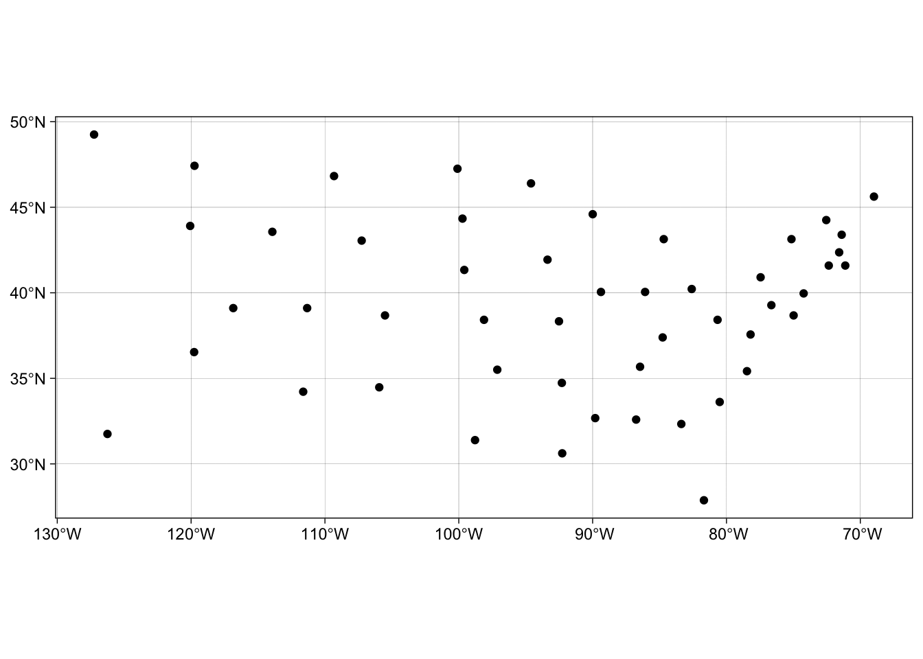
Simple feature collection with 50 features and 1 field
Geometry type: POINT
Dimension: XY
Bounding box: xmin: -127.25 ymin: 27.8744 xmax: -68.9801 ymax: 49.25
Geodetic CRS: NAD83
First 10 features:
name geometry
1 Alabama POINT (-86.7509 32.5901)
2 Alaska POINT (-127.25 49.25)
3 Arizona POINT (-111.625 34.2192)
4 Arkansas POINT (-92.2992 34.7336)
5 California POINT (-119.773 36.5341)
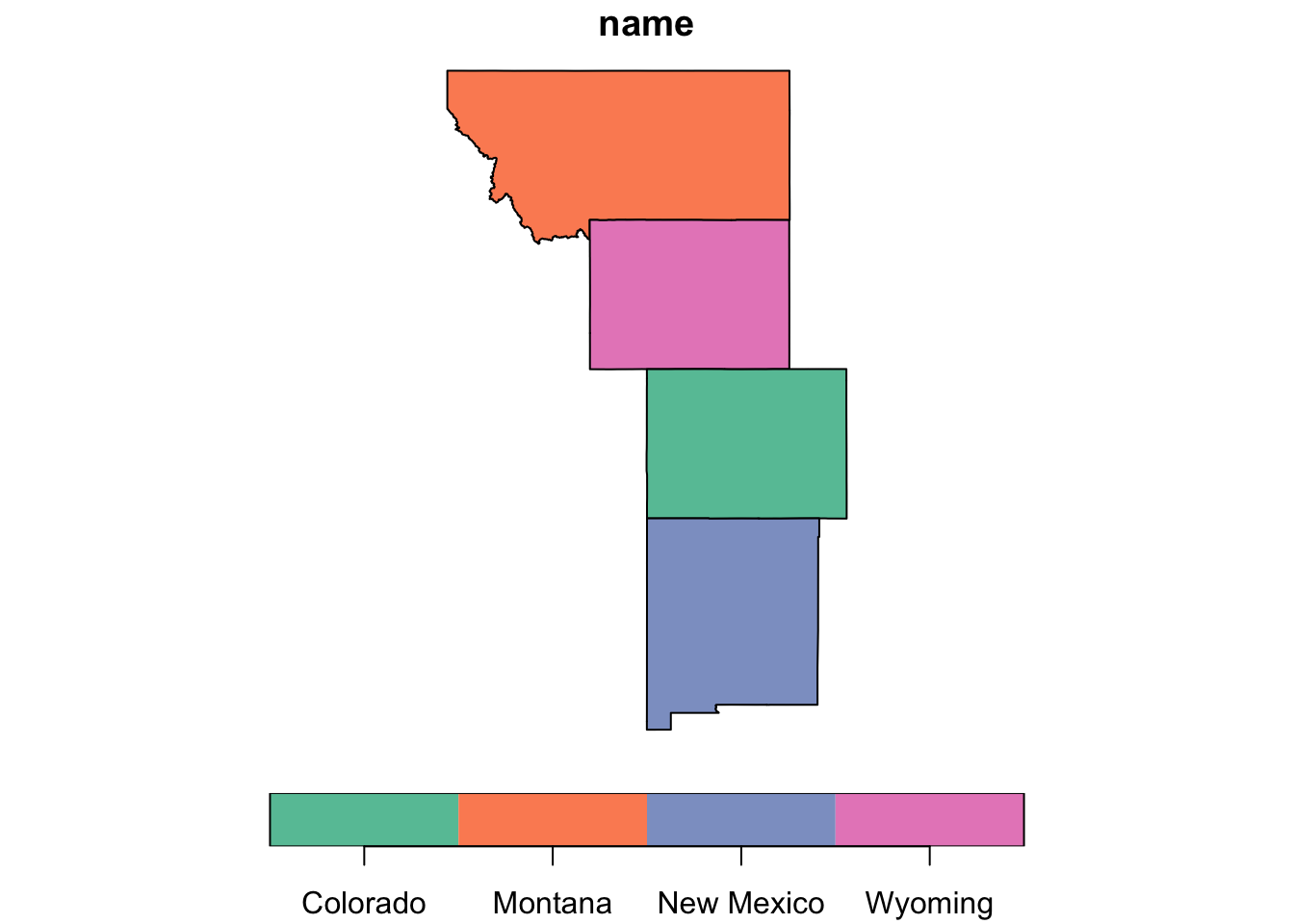
6 Colorado POINT (-105.513 38.6777)
7 Connecticut POINT (-72.3573 41.5928)
8 Delaware POINT (-74.9841 38.6777)
9 Florida POINT (-81.685 27.8744)
10 Georgia POINT (-83.3736 32.3329)
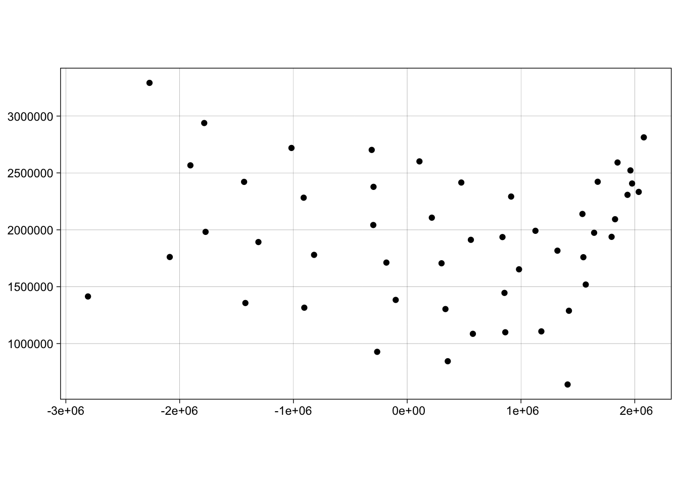
# Projected Coordinate System (PCS)# st_transforms converts from one reference system to another(df_sf_pcs =st_transform(df_sf_gcs, 5070))
Simple feature collection with 50 features and 1 field
Geometry type: POINT
Dimension:     XY
Bounding box:  xmin: -2805703 ymin: 640477 xmax: 2079664 ymax: 3291437
Projected CRS: NAD83 / Conus Albers
First 10 features:
          name                  geometry
1      Alabama  POINT (862043.5 1099545)
2       Alaska  POINT (-2264853 3291437)
3      Arizona  POINT (-1422260 1356663)
4     Arkansas  POINT (336061.5 1303543)
5   California  POINT (-2086972 1760961)
6     Colorado POINT (-818480.9 1779785)
7  Connecticut   POINT (1936213 2307450)
8     Delaware   POINT (1796466 1938236)
9      Florida    POINT (1409814 640477)
10     Georgia   POINT (1179012 1107322)
# Three most populous cities in the USA(big3 = cities |>select(city, population) |>slice_max(population, n =3))
Simple feature collection with 3 features and 2 fields
Geometry type: POINT
Dimension:     XY
Bounding box:  xmin: -2032604 ymin: 1468468 xmax: 1833394 ymax: 2178657
Projected CRS: NAD83 / Conus Albers
# A tibble: 3 × 3
  city        population           geometry
  <chr>            <dbl>        <POINT [m]>
1 New York      18832416  (1833394 2178657)
2 Los Angeles   11885717 (-2032604 1468468)
3 Chicago        8489066 (684628.5 2122697)
# Fort Collins(foco =filter(cities, city =="Fort Collins") |>select(city, population))
Simple feature collection with 1 feature and 2 fields
Geometry type: POINT
Dimension:     XY
Bounding box:  xmin: -760147.5 ymin: 1984621 xmax: -760147.5 ymax: 1984621
Projected CRS: NAD83 / Conus Albers
# A tibble: 1 × 3
  city         population            geometry
  <chr>             <dbl>         <POINT [m]>
1 Fort Collins     339256 (-760147.5 1984621)
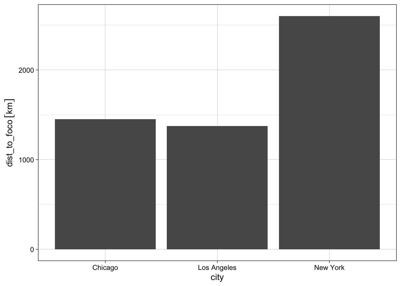
# Distance from foco to population centersst_distance(big3, foco)
It is returned as a matrix, even though foco only had one row
This second point highlights a useful feature of st_distance, namley, its ability to return distance matrices between all combinations of features in x and y.
units review
While units are useful, they are not always the preferred units. By default, the units measurement is defined by the projection. For example:
st_crs(big3)$units
[1] "m"
Units can be converted using units::set_units. For example, ‘m’ can be converted to ‘km’:
You might have noticed the data type of the st_distance objects are an S3 class of units. Sometimes, this class can cause problems when trying to using it with other classes or methods:
big3$dist_to_foco +4
Error in Ops.units(big3$dist_to_foco, 4): both operands of the expression should be "units" objects
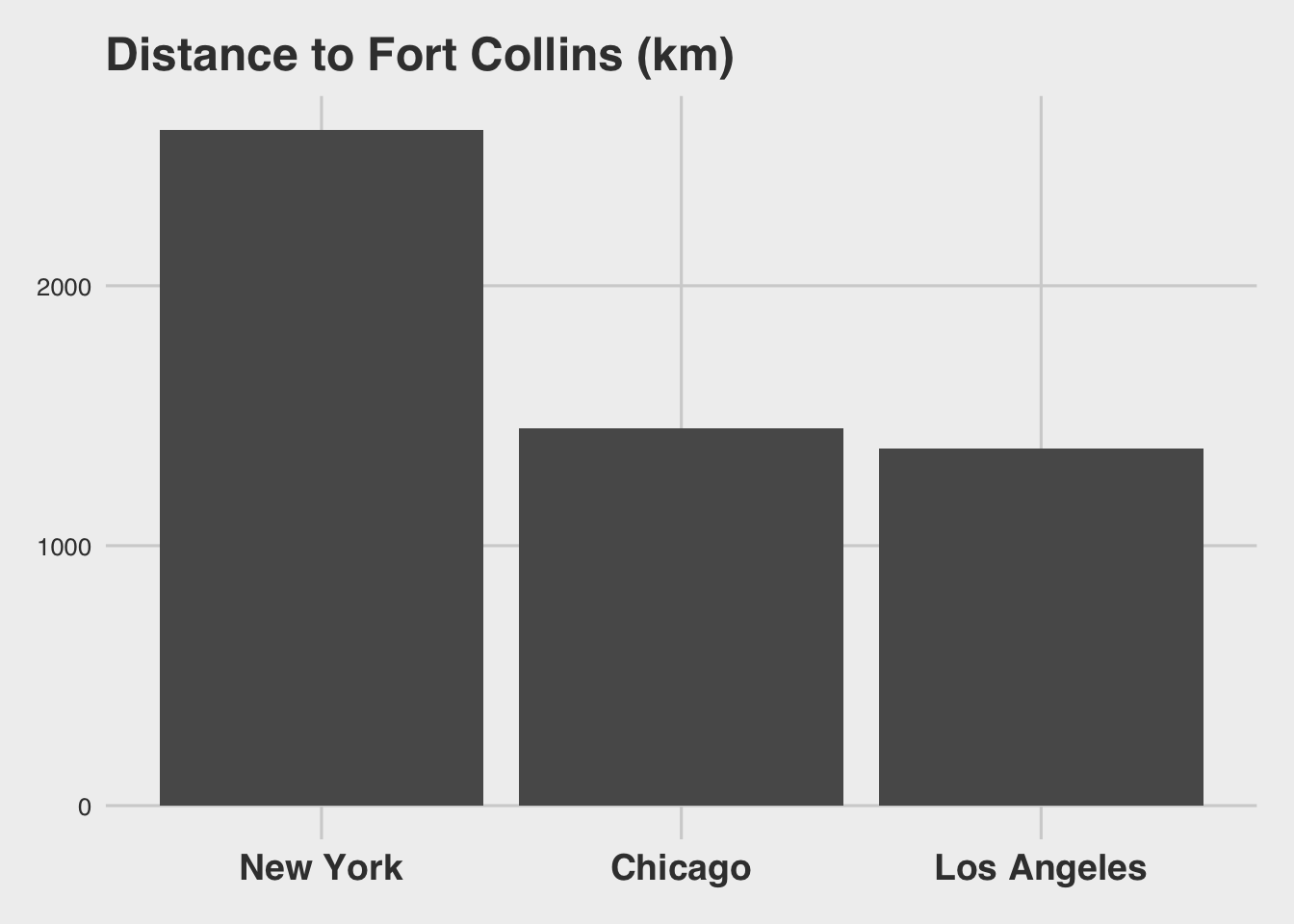
ggplot(data = big3) +geom_col(aes(x = city, y = dist_to_foco)) +theme_linedraw()
In these cases, the units class can be dropped with units::drop_units
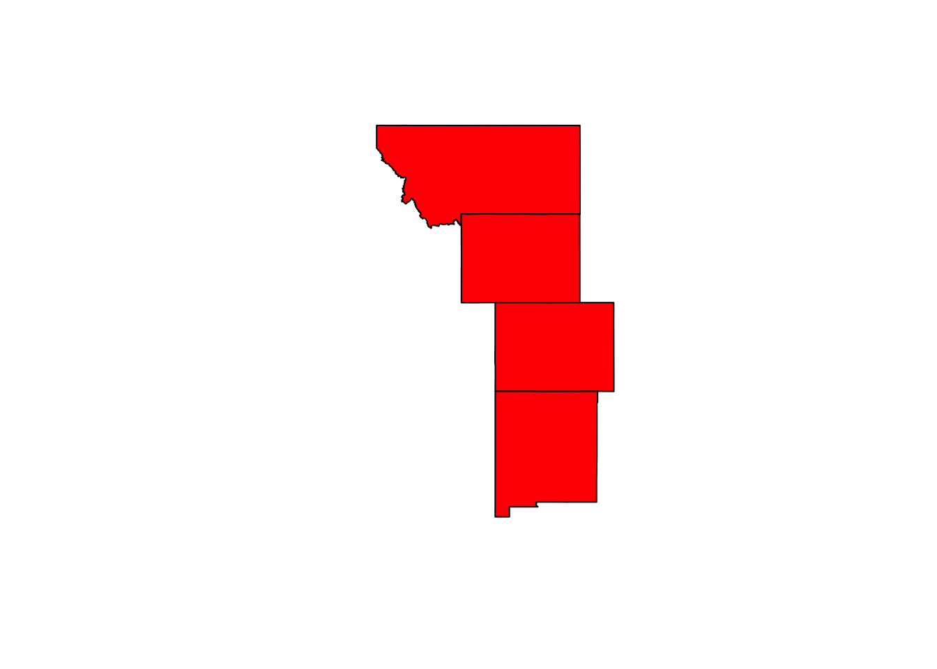
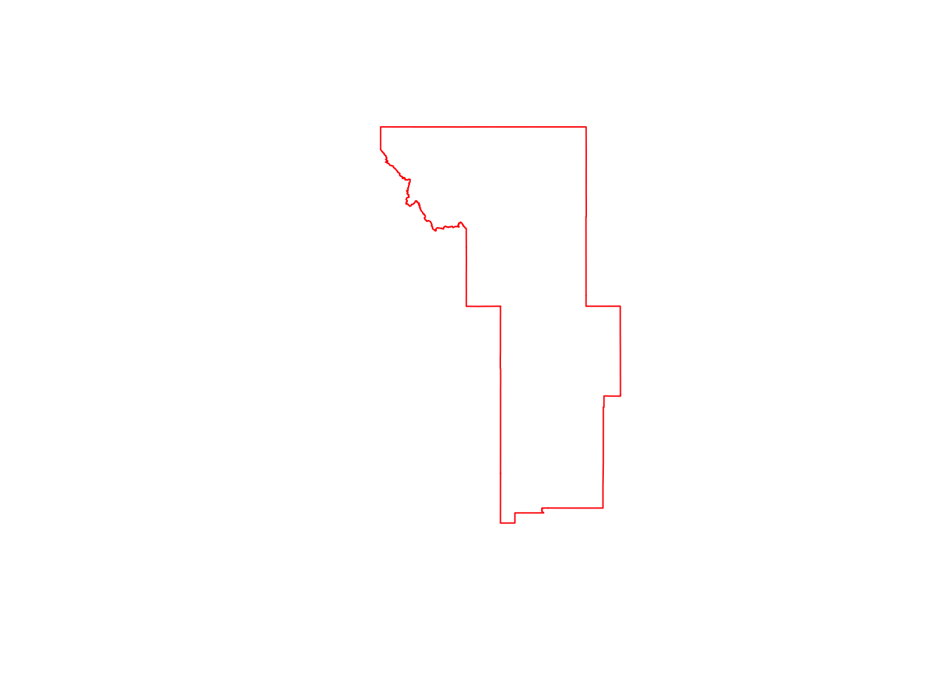
# Combine Geometriesline_wc =st_cast(unioned_wc, "MULTILINESTRING")plot(line_wc, col ="red")
Question 3:
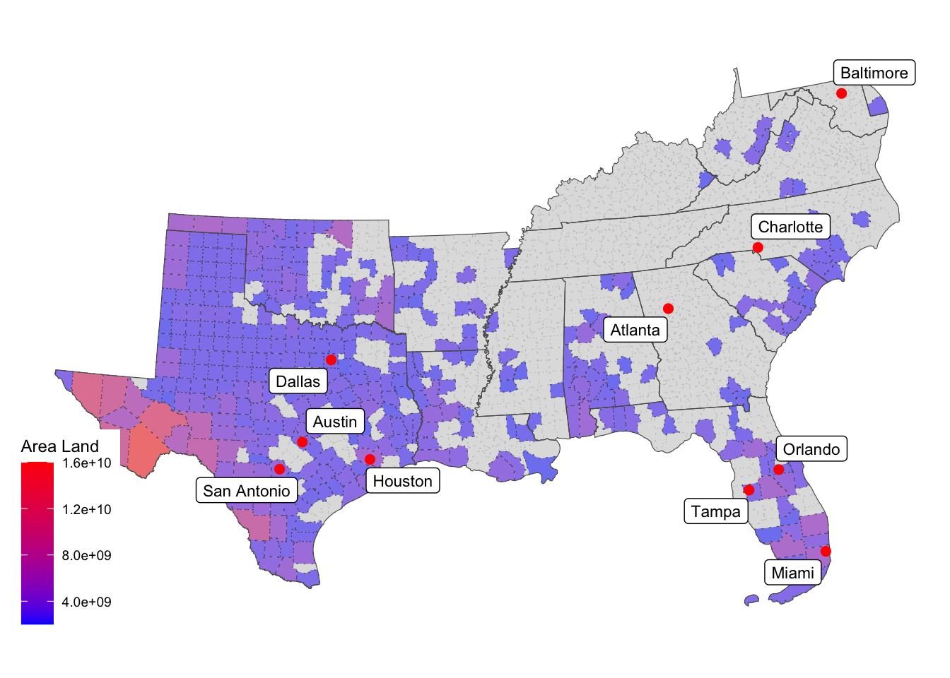
In this section you will extend your growing ggplot skills to handle spatial data using ggrepl to label significant features; gghighlight to emphasize important criteria; and scaled color/fill to create chloropleth represnetations of variables. Below is some example code to provide an example of these tools in action:
Get some data (review)
# Define a state/region classifier and select the southern statesstate.of.interest <-data.frame(state = state.name, region = state.region) |>filter(region =="South") |>pull(state)# Get USA states in the southern region and transform to EPSG:5070state = AOI::aoi_get(state ="conus") |>filter(name %in% state.of.interest) |>st_transform(5070)# Get USA counties in the southern region and transform to EPSG:5070counties = AOI::aoi_get(state ="conus", county ='all') |>filter(state_name %in% state.of.interest) |>st_transform(5070)# Get the 10 most populous cities in the southern region and transform to EPSG:5070sub_cities = cities |>filter(state_name %in% state.of.interest) |>slice_max(population, n =10) |>st_transform(5070)
Map
ggplot() +# Add districts with a dashed line (lty = 3), # a color gradient from blue to red based on land_area, # and a fill aplha of 0.5geom_sf(data = counties, aes(fill = land_area), lty =3, alpha = .5) +scale_fill_gradient(low ='blue', high ="red") +# Highlight (keep blue) only those districts witn a land area > 5e10gghighlight(land_area >2e9) +# Add the state borders with a thicker line and no fillgeom_sf(data = state, size =1, fill ="NA") +# Add the citiesgeom_sf(data = sub_cities, size=2, color ="red") +# Add labels to the cities ggrepel::geom_label_repel(data = sub_cities,aes(label = city, geometry = geometry),stat ="sf_coordinates",size =3) +labs(fill ="Area Land") + ggthemes::theme_map()