Lab 4: LTER Network Data

Introduction to Statistics in R

This lab will walk us through some basic statistical tests in R, including chi-square, t-tests, and correlation tests. We will use data from the Long-Term Ecological Research (LTER) Network, which is a collaborative effort involving more than 2000 scientists and students investigating ecological processes over long temporal and broad spatial scales. The basics of this lab were adopted from a previous version of this course. This qmd for this lab can be downloaded here. Please download it into the repo of your choice and open it in RStudio to work through this lab:

Part 1: Univariate and Bivariate Statistics

In this portion of the lab you will be introduced to the process of conducting statistical tests in R, specifically chi-square, t-tests, and correlation tests. These are commonly used for univariate and bivariate data.

Uni- vs bi- variate data

Univariate data consists of observations on a single variable. It describes one characteristic of a dataset without considering relationships between variables. Examples include:
- The heights of students in a class
- The daily temperature of a city
- The number of books read by individuals in a year

Bivariate data involves observations on two variables and explores the relationship between them. It is used to analyze correlations or dependencies. Examples include:
- The relationship between students’ study time and their exam scores
- The correlation between temperature and ice cream sales
- The effect of age on income level

To learn about this statistical tests, we will use data for cutthroat trout and salamander length and weights collected in Mack Creek, which is in the Andrews Forest Long-Term Ecological Research (LTER) facility in Oregon in the Cascade Mountains. Specifically, these data were collected in different forest treatments: clear cut or old growth.

First, to access the dataset(s) you will be using today install the lterdatasampler package (remotes is needed because lterdatasampler has to be installed from GitHub)

Code

remotes::install_github("lter/lterdatasampler")

Now load in the libraries needed for this lab:

Code

library(tidyverse)
library(ggpubr)
library(lterdatasampler)
library(car)
library(visdat)

Then run the following line of code to retrieve the and_vertebrates data set and bring it into your R session:

Code

?and_vertebrates

Explore the dataset

To start, we’ll begin looking at the and_vertebrates dataset. Start this section with some EDA to understand its structure, variables and data types:

Code

# View the data structure
glimpse(and_vertebrates)

Rows: 32,209
Columns: 16
$ year        <dbl> 1987, 1987, 1987, 1987, 1987, 1987, 1987, 1987, 1987, 1987…
$ sitecode    <chr> "MACKCC-L", "MACKCC-L", "MACKCC-L", "MACKCC-L", "MACKCC-L"…
$ section     <chr> "CC", "CC", "CC", "CC", "CC", "CC", "CC", "CC", "CC", "CC"…
$ reach       <chr> "L", "L", "L", "L", "L", "L", "L", "L", "L", "L", "L", "L"…
$ pass        <dbl> 1, 1, 1, 1, 1, 1, 1, 1, 1, 1, 1, 1, 1, 1, 1, 1, 1, 1, 1, 1…
$ unitnum     <dbl> 1, 1, 1, 1, 1, 1, 1, 1, 1, 1, 1, 1, 1, 1, 1, 1, 2, 2, 2, 2…
$ unittype    <chr> "R", "R", "R", "R", "R", "R", "R", "R", "R", "R", "R", "R"…
$ vert_index  <dbl> 1, 2, 3, 4, 5, 6, 7, 8, 9, 10, 11, 12, 13, 14, 15, 16, 1, …
$ pitnumber   <dbl> NA, NA, NA, NA, NA, NA, NA, NA, NA, NA, NA, NA, NA, NA, NA…
$ species     <chr> "Cutthroat trout", "Cutthroat trout", "Cutthroat trout", "…
$ length_1_mm <dbl> 58, 61, 89, 58, 93, 86, 107, 131, 103, 117, 100, 127, 99, …
$ length_2_mm <dbl> NA, NA, NA, NA, NA, NA, NA, NA, NA, NA, NA, NA, NA, NA, NA…
$ weight_g    <dbl> 1.75, 1.95, 5.60, 2.15, 6.90, 5.90, 10.50, 20.60, 9.55, 13…
$ clip        <chr> "NONE", "NONE", "NONE", "NONE", "NONE", "NONE", "NONE", "N…
$ sampledate  <date> 1987-10-07, 1987-10-07, 1987-10-07, 1987-10-07, 1987-10-0…
$ notes       <chr> NA, NA, NA, NA, NA, NA, NA, NA, NA, NA, NA, NA, NA, NA, NA…

Code

vis_dat(and_vertebrates)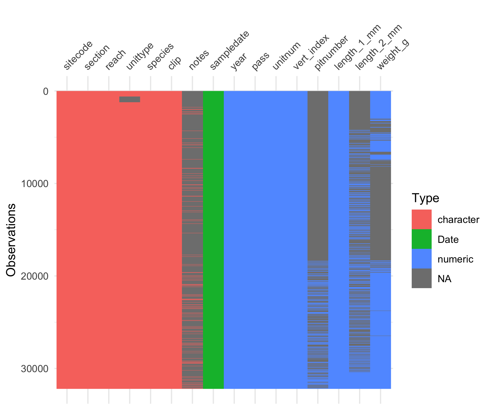

Code

# Explore the metadata in the Help pane
?and_vertebrates

This data set contains length and weight observations for three aquatic species in clear cut and old growth coniferous forest sections of Mack Creek in HJ Andrews Experimental Forest in Oregon. The three species are Cutthroat trout, Coastal giant salamander and Cascade torrent salamander.

Chi-square - Categorical Analysis

When you are working with two categorical variables, the statistical test you use is a Chi-square test. This test helps identify a relationship between your two categorical variables.

For example, we have two categorical variables in the and_vertebrates data set:

section = two forest sections, clear cut (CC) and old growth (OG)
unittype = stream channel unit classification type (C = cascade, I = riffle, IP = isolated pool (not connected to channel), P = pool, R = rapid, S = step (small falls), SC = side channel, NA = not sampled by unit)

Lets focus this question on Cutthroat trout. First explore the abundance of cutthroat trout in different channel types, using the count() function to return the total count/number of observations in each group - making sure to limit your analysis to “Cutthroat trout”.

Code

and_vertebrates |> 
  filter(species == "Cutthroat trout") |> 
  count(unittype)

# A tibble: 8 × 2
  unittype     n
  <chr>    <int>
1 C        11419
2 I           23
3 IP         105
4 P         5470
5 R          420
6 S            9
7 SC        2377
8 <NA>       610

This output tells us that there are quite a few observations with the NA category, meaning channel type was unknown or not recorded. Let’s edit the workflow above slightly, using drop_na() to remove any rows within a specified column (or columns) that have NA values:

Code

and_vertebrates |> 
  filter(species == "Cutthroat trout") |> 
  drop_na(unittype) |> 
  count(unittype)

# A tibble: 7 × 2
  unittype     n
  <chr>    <int>
1 C        11419
2 I           23
3 IP         105
4 P         5470
5 R          420
6 S            9
7 SC        2377

This returns just about the same data frame as the first method, but now with the NA category removed because it dropped any observations that were NA for unittype.

From this we also observe that the highest Cutthroat trout abundances are found in cascade (C), pool (P), and side channel (SC) habitats.

Now, our question expands beyond this one categorical variable (channel type) and we want to know if abundance is affected by both channel and and forest type (section). Here, our null hypothesis is that forest and channel type are independent. To test this, we use the chisq.test() to carry out a chi-square test, but first we have to reformat our data into a contingency table.

A contingency table is in matrix format, where each cell is the frequency (in this case seen as abundance) of Cutthroat trout in each combination of categorical variables (forest type and channel unit). We can create a contingency table with the table() function. For this analysis, lets also keep just the 3 most abundant unit types for Cutthroat trout (C, P and SC).

Code

# First clean the dataset to create the contingency table from
trout_clean <- and_vertebrates  |>  
  #filter Cutthroat trout
  filter(species == "Cutthroat trout") |> 
  # lets test using just the 3 most abundant unittypes
  filter(unittype %in% c("C", "P", "SC")) |> 
  # drop NAs for both unittype and section
  drop_na(unittype, section)

cont_table <- table(trout_clean$section, trout_clean$unittype)

To execute the Chi-square test does not take that much code, but it is important to note that by default, chisq.test() assumes the null hypothesis is that all frequencies have equal probability. If you have different pre-conceived frequency probabilities for your data you have to define those within the chisq.test() function.

Code

chisq.test(cont_table)


    Pearson's Chi-squared test

data:  cont_table
X-squared = 188.68, df = 2, p-value < 2.2e-16

Looking at these results, we see an extremely small p-valuetelling us there is a significant relationship between forest type and channel unit (i.e., we rejected our null hypothesis).

Lets look at the abundance distribution visually:

Code

trout_clean  |>  
  count(unittype, section)  |>  
  ggpubr::ggbarplot(x = 'unittype', y = 'n', 
                    fill = 'section', 
                    palette = c("#00AFBB", "#E7B800"),
                    add = "mean_se")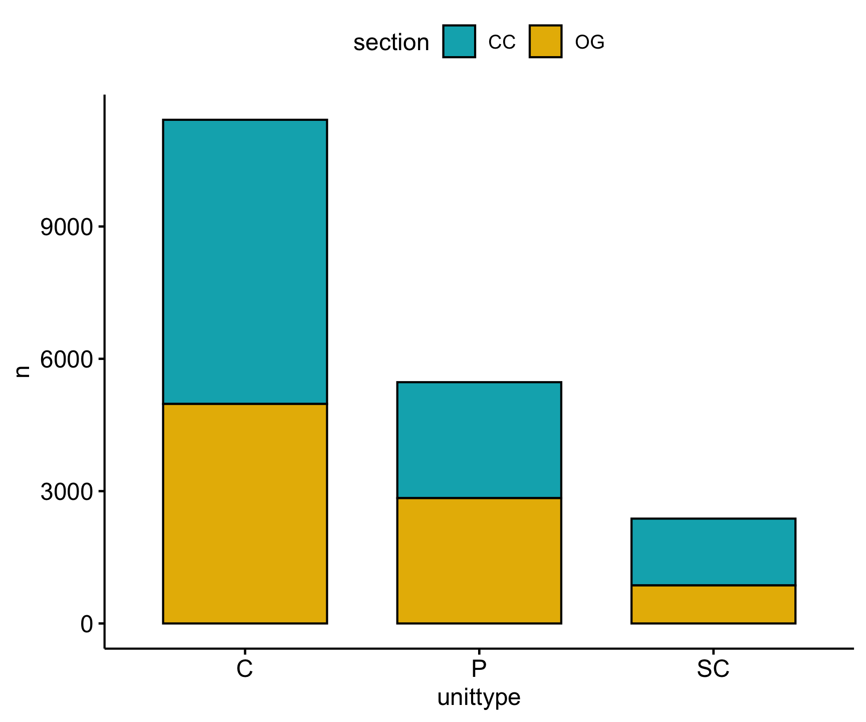

t-test - Compare two means

Previous work has shown that forest harvesting practics can impact aquatic vertebrate biomass (Kaylor & Warren 2017). Using the and_vertebrates data set we can investigate this by comparing weight to forest type (clear cut or old growth). This involves a test to compare the means (average weight) among two groups (clear cut and old growth forests) using a t-test.

Let’s focus on conducting this test for Cutthroat trout. We can use the same trout_clean data set we made earlier so long as we drop all NAs in weight_g. Once this is done, we can visualize the differences in weight among forest type with a boxplot:

Code

trout_clean |> 
  drop_na(weight_g) |> 
  ggpubr::ggviolin(x = "section", 
                   y     = "weight_g", 
                   add   = "boxplot",
                   color = "section",
                   palette = c("#00AFBB", "#E7B800"))

We don’t see too much of a difference based on this visual, but we need to conduct the statistical test to verify. Before we dive into the statistical t-test, we must check our assumptions!

Test Assumptions: A t-test assumes the variance of each group is equal and the data are normally distributed.

Equal Variance We can test for equal variances with the function var.test(), where the null hypothesis is that the variances are equal. In this step, we need two vectors of the weights in each separate forest section. You can use pull() to convert a single column of a data frame/tibble to a vector, and we want to do this for clear cut and old growth forests.

Code

cc_weight <- trout_clean |> 
  filter(section == "CC") |> 
  pull(weight_g)

og_weight <- trout_clean |> 
  filter(section == "OG") |> 
  pull(weight_g)

var.test(cc_weight, og_weight)


    F test to compare two variances

data:  cc_weight and og_weight
F = 1.2889, num df = 6310, denom df = 5225, p-value < 2.2e-16
alternative hypothesis: true ratio of variances is not equal to 1
95 percent confidence interval:
 1.223686 1.357398
sample estimates:
ratio of variances 
          1.288892

The results of this test suggests the variances are not equal. How do we know this? If you can’t remember, please refresh your memory of the null hypothesis for the variance test and how to interpret the p-value.

Note

One option for data with unequal variances is to use the non parametric Welch t-test, which does not assume equal variances. We will explore this test later.

Normal Distribution A t-test mandates data with a normal distribtution. Here we can use a visual method to access the normality of the data:

Code

ggpubr::ggarrange(ggpubr::gghistogram(cc_weight, main = "Clear Cut"), 
                  ggpubr::gghistogram(og_weight, main = "Old Growth"))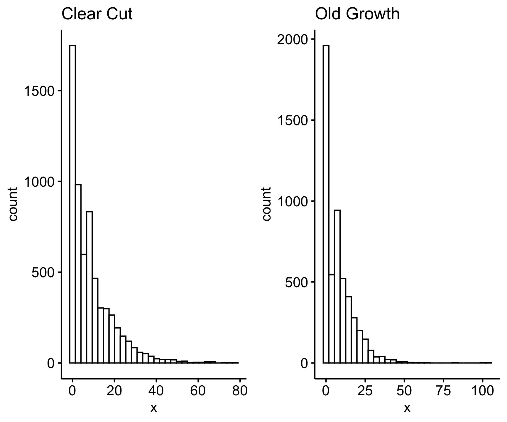

We can see from the histograms that the data are very right skewed. When we see a heavy right skew, we know a log transform can help normalize the data. Let’s check the variances like we did before using the log transformed values:

Code

var.test(log(cc_weight), log(og_weight))


    F test to compare two variances

data:  log(cc_weight) and log(og_weight)
F = 1.0208, num df = 6310, denom df = 5225, p-value = 0.4374
alternative hypothesis: true ratio of variances is not equal to 1
95 percent confidence interval:
 0.9691443 1.0750427
sample estimates:
ratio of variances 
          1.020787

Now we have a much higher p-value, indicating support for the null that the variances of log-transformed data are equal. So we can use the default t.test() test which assumes equal variances, but only on a log transformed weight variable.

The t.test() function takes in your dependent (in our case trout weight) and independent (forest type) variables as vectors. The order of the variables in the t.test() function is {dependent variable} ~ {independent variable}. We use the ~ to specify a model, telling the test we want to know if weight varies by forest section.

Remember we also want to log transform the weight values and then specify that our variances are equal since we confirmed that with var.test() above, so the final t.test() call would be this:

Code

t.test(log(trout_clean$weight_g) ~ trout_clean$section, var.equal = TRUE)


    Two Sample t-test

data:  log(trout_clean$weight_g) by trout_clean$section
t = 2.854, df = 11535, p-value = 0.004324
alternative hypothesis: true difference in means between group CC and group OG is not equal to 0
95 percent confidence interval:
 0.02222425 0.11969560
sample estimates:
mean in group CC mean in group OG 
        1.457042         1.386082

The output of this test gives us the test statistics, p-value, and the means for each of our forest groups. Given the p-value of 0.0043, we reject the null hypothesis (mean Cutthroat weight is the same in clear cut and old growth forest sections), and looking at our results - specifically the means - we can conclude that Cutthroat trout weight was observed to be significantly higher in clear cut forests compared to old growth forests. Remember that the mean weight values are log transformed and not the raw weight in grams. The relationship can still be interpreted the same, but you will want to report the means from the raw weight data.

How does this relate to the original hypothesis based on the graph we made at the beginning of this section?

Welch Two Sample t-test

Alternatively, instead of transforming our variable we can change the default t.test() argument by specifying var.equal = FALSE, which will then conduct a Welch t-test, which does not assume equal variances among groups.

Code

t.test(trout_clean$weight_g ~ trout_clean$section, var.equal = FALSE)


    Welch Two Sample t-test

data:  trout_clean$weight_g by trout_clean$section
t = 4.5265, df = 11491, p-value = 6.056e-06
alternative hypothesis: true difference in means between group CC and group OG is not equal to 0
95 percent confidence interval:
 0.4642016 1.1733126
sample estimates:
mean in group CC mean in group OG 
        8.988807         8.170050

While using a slightly different method, our conclusions are the same, finding that Cutthroat trout had significantly higher weights in clear cut forests than old growth.

Note: In the t.test() function you can add paired = TRUE to conduct a paired t-test. These are for cases when the groups are ‘paired’ for each observation, meaning each group/treatment was applied to the same individual, such as experiments that test the impact of a treatment, with measurements before and after the experiment.

Correlation - Assess relationships

To assess the relationship between two continuous variables, you use a correlation test, which is the cor.test() function. Correlation tests assess the presence of a significant relationship and the strength of each relationship (i.e., the correlation coefficient). There are multiple correlation methods you can use with this function but by default, it uses the Pearson correlation method which assumes your data are normally distributed and there is a linear relationship. If these assumptions are not met, you can use a Spearman Rank correlation test, a non-parametric test that is not sensitive to the variable distribution. To use this method, specify spearman for method.

For our and_vertebrates data set, we can test the relationship of length and weight. Let’s test the hypothesis that body length is positively correlated with weight, such that longer individuals will also weigh more, specifically looking at the Coastal Giant salamander.

First let’s clean our data set to just include the Coastal giant salamander and remove missing values for length and weight.

Code

sally_clean <- and_vertebrates |> 
  filter(species == "Coastal giant salamander") |> 
  drop_na(length_2_mm, weight_g)

Testing Assumptions

Let’s look at the distribution of these variables first:

Code

ggarrange(gghistogram(sally_clean$length_2_mm, title = "Length"),
gghistogram(sally_clean$weight_g, title = "Weight"))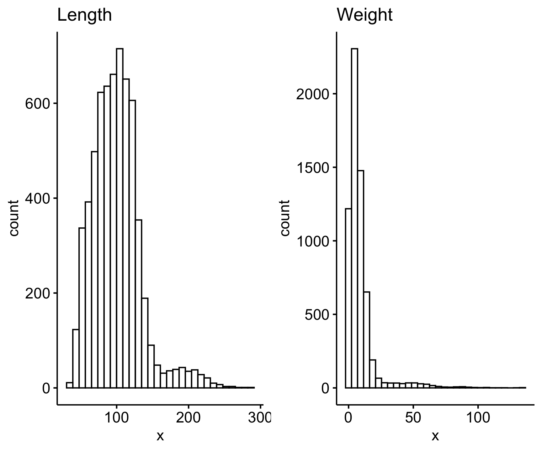

They both look pretty skewed, therefore likely not normally distributed. We can statistically test if a variable fits a normal distribution with the shapiro.test() function, which is the Shapiro-Wilk normality text. However note that this function only runs for 5,000 observations or less, so we will test for normality for a sample of our sally_clean data set:

Code

s <- sally_clean |> 
  slice_sample(n = 5000) 

shapiro.test(s$length_2_mm)


    Shapiro-Wilk normality test

data:  s$length_2_mm
W = 0.93513, p-value < 2.2e-16

Code

shapiro.test(s$weight_g)


    Shapiro-Wilk normality test

data:  s$weight_g
W = 0.57988, p-value < 2.2e-16

The null hypothesis of the Shapiro-Wilk normality test is that the variable is normally distributed, so a significant p-value less than 0.05 (as we see for both of our variables here) tells use that our data does not fit a normal distribution.

Therefore we have two options as we did with our earlier t-test example: transform the variables or use the non-parametric test.

Variable transformation

Lets try the first option by log transforming our variables, first viewing the log-transformed distribution for each variable.

Code

ggarrange(
 gghistogram(log(sally_clean$length_2_mm), title = "Length"), 
 gghistogram(log(sally_clean$weight_g), title = "Weight") )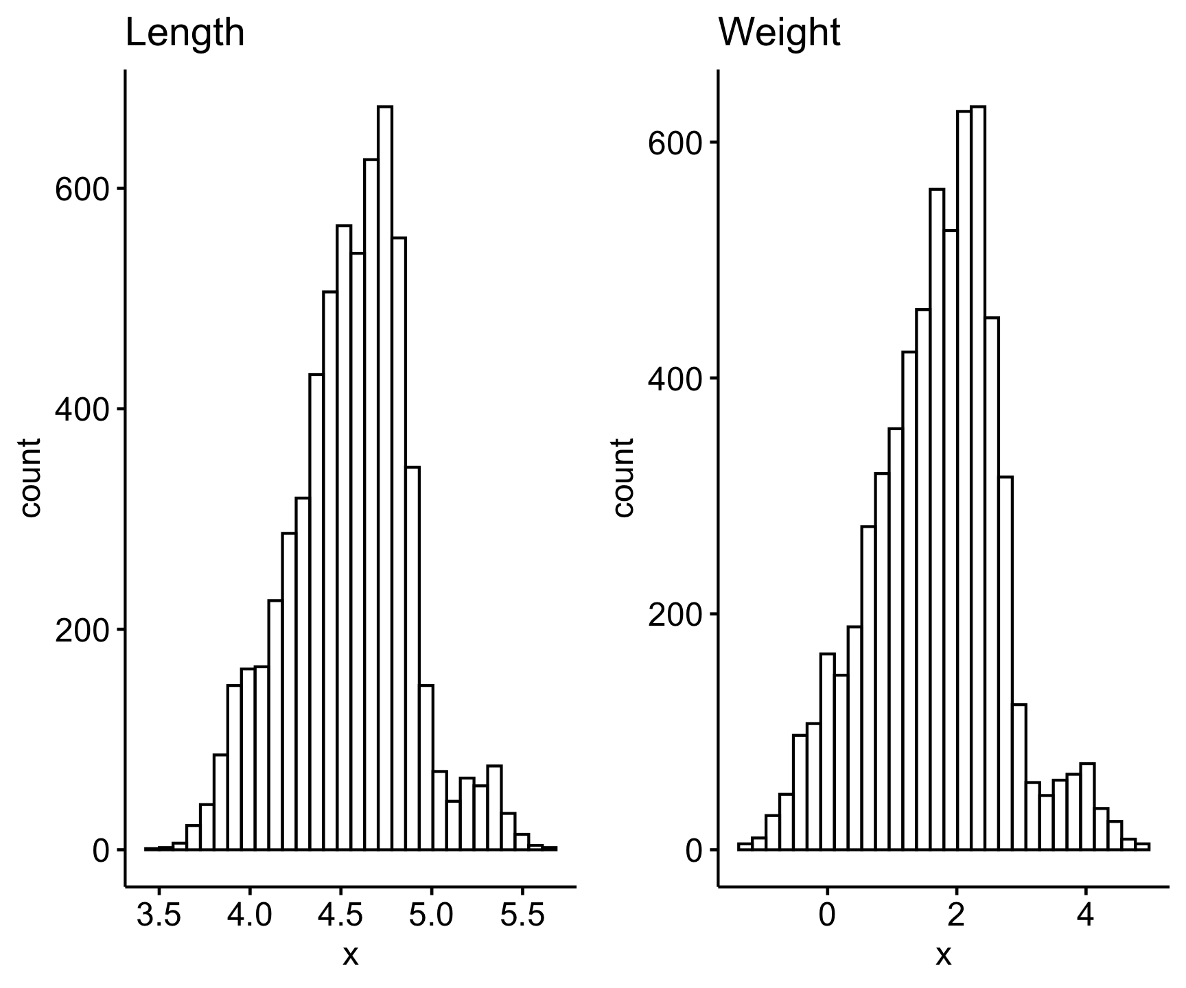

Since the log-transformed data look normally distributed (note that we can test using the Shapiro-Wilk normality test on the log-transformed data), we can use the Pearson’s correlation test (the default for cor.test()). All we need to add to the cor.test() argument is the two variables of our sally_clean data set we want to test a relationship for, and keep them log-transformed since those distributions looked closer to a normal distribution (visually at least).

Code

cor.test(log(sally_clean$length_2_mm), log(sally_clean$weight_g))


    Pearson's product-moment correlation

data:  log(sally_clean$length_2_mm) and log(sally_clean$weight_g)
t = 402.85, df = 6229, p-value < 2.2e-16
alternative hypothesis: true correlation is not equal to 0
95 percent confidence interval:
 0.9804036 0.9822403
sample estimates:
      cor 
0.9813443

From these results we see a very small p-value, meaning there is a significant association between the two, and a correlation coefficient of 0.98, representing a strong, positive correlation.

Let’s look at this correlation visually:

Code

sally_clean |> 
  mutate(log_length = log(length_2_mm), log_weight = log(weight_g)) |> 
  ggscatter(x = 'log_length', 
            y = 'log_weight', 
            alpha = .35,
            add = "loess")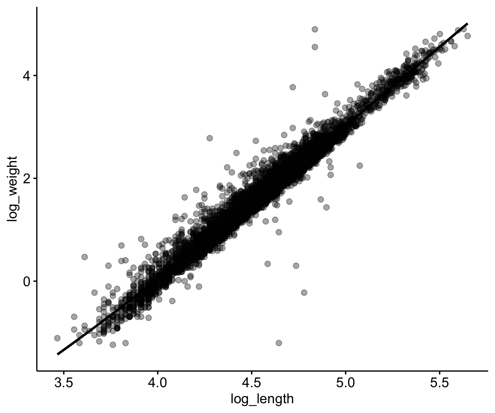

Spearman Correlation Test

Let’s now perform the correlation test again but keeping our raw data and instead specifying method = 'spearman', as the Spearman test is better for non-parametric and non-linear data sets.

Code

cor.test(sally_clean$length_2_mm, sally_clean$weight_g, method = "spearman")


    Spearman's rank correlation rho

data:  sally_clean$length_2_mm and sally_clean$weight_g
S = 819296957, p-value < 2.2e-16
alternative hypothesis: true rho is not equal to 0
sample estimates:
      rho 
0.9796802

These results also represent a significant, positive relationship between length and weight for the Coastal Giant salamander, with a very high correlation coefficient.

Exercises: Part 1

Each question requires you to carry out a statistical analysis to test some hypothesis related to the and_vertebrates data set. To answer each question fully:

Include the code you used to clean the data and conduct the appropriate statistical test. (Including the steps to assess and address your statistical test assumptions).
Report the findings of your test in proper scientific format (with the p-value in parentheses).

1. Conduct a chi-square test similar to the one carried out above, but test for a relationship between forest type (section) and channel unit (unittype) for Coastal giant salamander abundance. Keep all unittypes instead of filtering any like we did for the Cutthroat trout (10 pts.)

2. Test the hypothesis that there is a significant difference in species biomass between clear cut and old growth forest types for the Coastal Giant salamander. (10 pts.)

3. Test the correlation between body length (snout to fork length) and body mass for Cutthroat trout. (Hint: run ?and_vertebrates to find which length variable represents snout to fork length) (10 pts.)

Part 2: Multivariate Statistics

In this part you will be introduced to statistical tests for dealing with more complex data sets, such as when you need to compare across more than two groups (ANOVA) or assess relationships in the form of an equation to predict response variables given single or multiple predictors (Regression).

We need to install one new package for today to use a specific statistical test. This package is called car. Follow the steps below to install the package, and then read in your libraries and data set for the lesson.

Code

#install the car package
install.packages("car")
??car

Code

# data set
data("pie_crab")

Explore the Data set

This data set consists of Fiddler crab body size measured in salt marshes from Florida to Massachusetts during summer 2016 at Plum Island Ecosystem LTER.

Code

glimpse(pie_crab)

Rows: 392
Columns: 9
$ date          <date> 2016-07-24, 2016-07-24, 2016-07-24, 2016-07-24, 2016-07…
$ latitude      <dbl> 30, 30, 30, 30, 30, 30, 30, 30, 30, 30, 30, 30, 30, 30, …
$ site          <chr> "GTM", "GTM", "GTM", "GTM", "GTM", "GTM", "GTM", "GTM", …
$ size          <dbl> 12.43, 14.18, 14.52, 12.94, 12.45, 12.99, 10.32, 11.19, …
$ air_temp      <dbl> 21.792, 21.792, 21.792, 21.792, 21.792, 21.792, 21.792, …
$ air_temp_sd   <dbl> 6.391, 6.391, 6.391, 6.391, 6.391, 6.391, 6.391, 6.391, …
$ water_temp    <dbl> 24.502, 24.502, 24.502, 24.502, 24.502, 24.502, 24.502, …
$ water_temp_sd <dbl> 6.121, 6.121, 6.121, 6.121, 6.121, 6.121, 6.121, 6.121, …
$ name          <chr> "Guana Tolomoto Matanzas NERR", "Guana Tolomoto Matanzas…

Code

vis_dat(pie_crab)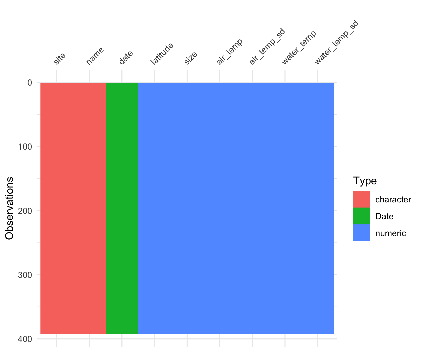

Learn more about each variable:

Code

?pie_crab

This data set provides a great opportunity to explore Bergmann’s rule: where organisms at higher latitudes are larger than those at lower latitudes. There are various hypotheses on what drives this phenomenon, which you can read more about in Johnson et al. 2019.

We have a continuous size variable (carapace width in mm), our dependent variable, and various predictor variables: site (categorical), latitude (continuous), air temperature (continuous) and water temperature (continuous).

Let’s explore the sample size at each site and how many sites are in this data set

Code

# sample size per site
count(pie_crab, site)

# A tibble: 13 × 2
   site      n
   <chr> <int>
 1 BC       37
 2 CC       27
 3 CT       33
 4 DB       30
 5 GTM      28
 6 JC       30
 7 NB       29
 8 NIB      30
 9 PIE      28
10 RC       25
11 SI       30
12 VCR      30
13 ZI       35

We have 13 sites with ~30 individual male crabs measured at each site.

Let’s also check the range of our continuous variables:

Code

summary(pie_crab)

      date               latitude         site                size      
 Min.   :2016-07-24   Min.   :30.00   Length:392         Min.   : 6.64  
 1st Qu.:2016-07-28   1st Qu.:34.00   Class :character   1st Qu.:12.02  
 Median :2016-08-01   Median :39.10   Mode  :character   Median :14.44  
 Mean   :2016-08-02   Mean   :37.69                      Mean   :14.66  
 3rd Qu.:2016-08-09   3rd Qu.:41.60                      3rd Qu.:17.34  
 Max.   :2016-08-13   Max.   :42.70                      Max.   :23.43  
    air_temp      air_temp_sd      water_temp    water_temp_sd  
 Min.   :10.29   Min.   :6.391   Min.   :13.98   Min.   :4.838  
 1st Qu.:12.05   1st Qu.:8.110   1st Qu.:14.33   1st Qu.:6.567  
 Median :13.93   Median :8.410   Median :17.50   Median :6.998  
 Mean   :15.20   Mean   :8.654   Mean   :17.65   Mean   :7.252  
 3rd Qu.:18.63   3rd Qu.:9.483   3rd Qu.:20.54   3rd Qu.:7.865  
 Max.   :21.79   Max.   :9.965   Max.   :24.50   Max.   :9.121  
     name          
 Length:392        
 Class :character  
 Mode  :character

ANOVA

Our first question is if there is a significant difference in crab size among the 13 sites? Since we have a continuous response variable (size) and a categorical predictor (site) with > 2 groups (13 sites), we will use an ANOVA test.

Let’s first visualize the distribution of sizes for each site using a new visualization technique with ggplot called geom_jitter(). This function adds a small amount of variation to each point, so that all our points for each site are not stacked on top of each other.

Code

pie_crab |> 
  ggboxplot(x = 'site', y = 'size', col = 'site') +
  geom_jitter(size =.25) + 
  theme(legend.postition = "none")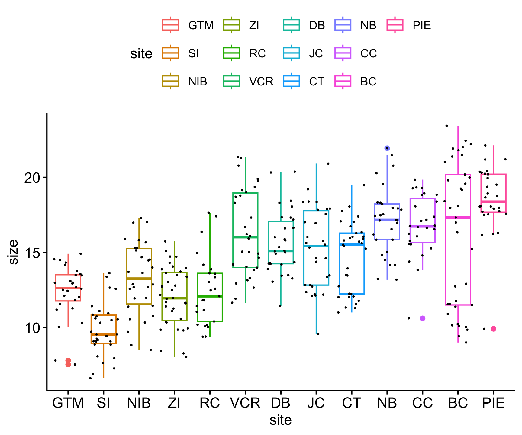

In doing this, it ;ooks like there are differences among sites, tempting us to test for statistical significance with the ANOVA test.

Assumptions

Normality

ANOVA assumes normal distributions within each group. We can utlize out nest/map approach to assess the normality of our data. We will use the Shapiro-Wilk normality test, which is a good test for small sample sizes.

Code

norms <- pie_crab |> 
  nest(data = -site) |>
  mutate(Shapiro = map(data, ~ shapiro.test(.x$size)),
         n = map_dbl(data, nrow),
         glance_shapiro = map(Shapiro, broom::glance)) |>
  unnest(glance_shapiro)

flextable::flextable(dplyr::select(norms, site, n, statistic, p.value)) |>
  flextable::set_caption("Shapiro-Wilk normality test for size at each site")

site	n	statistic	p.value
GTM	28	0.9007814	0.0119337484
SI	30	0.9705352	0.5539208550
NIB	30	0.9728297	0.6191340731
ZI	35	0.9744583	0.5765589900
RC	25	0.9315062	0.0941588802
VCR	30	0.9444682	0.1200262239
DB	30	0.9576271	0.2690631942
JC	30	0.9634754	0.3788327942
CT	33	0.9277365	0.0301785639
NB	29	0.9675367	0.4949587443
CC	27	0.9354659	0.0941803007
BC	37	0.8885721	0.0014402753
PIE	28	0.8489399	0.0008899392

In nearly all cases, the p-value > 0.01 (with the exception of BC and PIE), so we generally accept the null that this data does fit the normal distribution assumption across groups.

A residual value is computed for each observation as the difference between an individual value in a group and the mean of the group.

We can first compute the residuals from the ANOVA model using the aov() function. To carry out the ANOVA model, we specify the name of our continuous response (size) ~ (which you read as ‘by’) the name of our categorical predictor (site), and specify the data set name.

Code

(res_aov <- aov(size ~ site, data = pie_crab))

Call:
   aov(formula = size ~ site, data = pie_crab)

Terms:
                    site Residuals
Sum of Squares  2172.376  2626.421
Deg. of Freedom       12       379

Residual standard error: 2.632465
Estimated effects may be unbalanced

We can then pull out the residuals of this aov() model the same way we index columns with the $ operator. Let’s check the distribution visually and statistically.

Code

gghistogram(res_aov$residuals)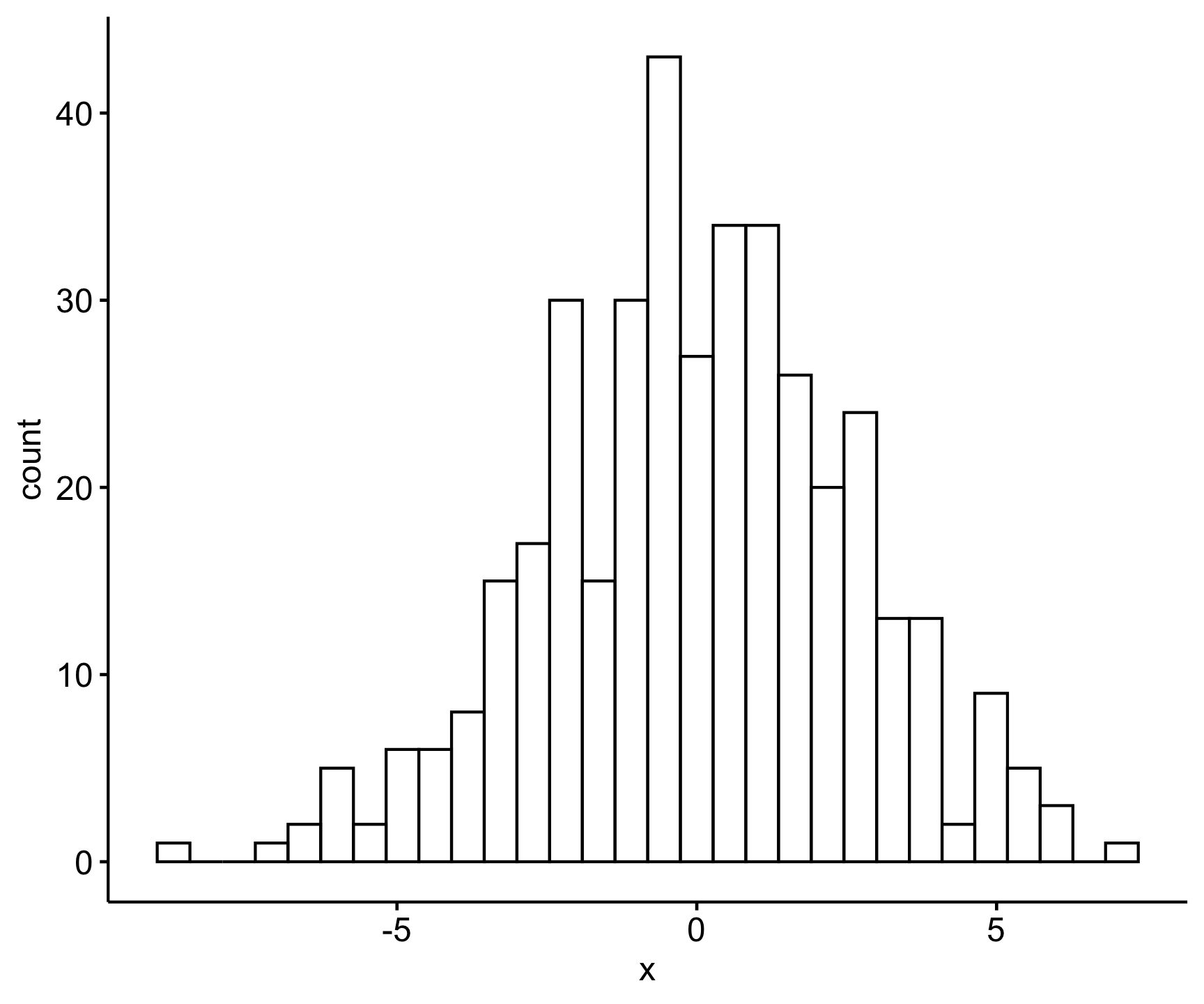

Code

shapiro.test(res_aov$residuals)


    Shapiro-Wilk normality test

data:  res_aov$residuals
W = 0.99708, p-value = 0.7122

This returns a p-value of 0.71, so we accept the null hypothessis that this data fits a normal distribution assumption.

Equal Variances

To test for equal variances among more than two groups, it is easiest to use a Levene’s Test. To use this test we need to install a new package called car, which you should have done at the beginning of this lesson.

Code

leveneTest(size ~ site, data = pie_crab)

Levene's Test for Homogeneity of Variance (center = median)
       Df F value    Pr(>F)    
group  12  9.2268 1.151e-15 ***
      379                      
---
Signif. codes:  0 '***' 0.001 '**' 0.01 '*' 0.05 '.' 0.1 ' ' 1

ANOVA

Similar to the var.test() function you’ve used before, the null hypothesis of the Levene’s test is that the variances are equal across all groups. Given this small p-value (denoted the the ‘Pr(>F)’ value) we confirm that the variances of our groups are not equal. Therefore we need to use a Welch ANOVA (oneway.test), which we specify by setting var.equal = FALSE:

Code

#perform Welch's ANOVA
oneway.test(size ~ site, data = pie_crab, var.equal = FALSE)


    One-way analysis of means (not assuming equal variances)

data:  size and site
F = 39.108, num df = 12.00, denom df = 145.79, p-value < 2.2e-16

Our results here are highly significant, meaning that at least one of our site means is significantly different from the others. However, ANOVA tests don’t tell us which sites are significantly different. To tell which sites are different, we need to use the Tukey’s HSD post-hoc test which gives us pairwise comparisons.

With 13 sites, it results in a lot of pairwise comparisons. For the next example, let’s simplify our analysis to just check for differences among 3 sites, choosing sites at the two latitude extremes and one in the middle. We’ll also need to rerun the ANOVA on the data subset since the Tukey’s HSD uses the ANOVA model. We know that the data meet the normality assumption, and we should recheck the equality assumption within our data subset.

Code

# Filter a subset of the sites
pie_sites <- pie_crab |> 
  filter(site %in% c("GTM", "DB", "PIE"))

# Check for equal variance
leveneTest(size ~ site, data = pie_sites)

Levene's Test for Homogeneity of Variance (center = median)
      Df F value Pr(>F)
group  2   0.548 0.5802
      83

Code

# Note that the variances are equal (p = 0.5802), so we can proceed with the ANOVA

# ANOVA for the data subset
pie_anova <- aov(size ~ site, data = pie_sites)

# View the ANOVA results 
summary(pie_anova)

            Df Sum Sq Mean Sq F value Pr(>F)    
site         2  521.5  260.75   60.02 <2e-16 ***
Residuals   83  360.6    4.34                   
---
Signif. codes:  0 '***' 0.001 '**' 0.01 '*' 0.05 '.' 0.1 ' ' 1

Post-hoc Tukey’s HSD test

From the ANOVA test, we find that at least one of our group means is significantly different from the others. Now we can use the TukeyHSD() function to test all the pairwise differences to see which groups are different from each other.

Code

TukeyHSD(pie_anova)

  Tukey multiple comparisons of means
    95% family-wise confidence level

Fit: aov(formula = size ~ site, data = pie_sites)

$site
             diff       lwr       upr   p adj
GTM-DB  -3.200786 -4.507850 -1.893722 3.0e-07
PIE-DB   2.899929  1.592865  4.206992 2.9e-06
PIE-GTM  6.100714  4.771306  7.430123 0.0e+00

This returns each combination of site comparisons and a p-value (the ‘p adj’ variable) for each.

Linear Regression

Let’s more directly test Bergmann’s rule by testing for a relationship between carapace width and latitude. Since our predictor (latitude) is a continuous variable, we can conduct a simple linear regression.

A note on assumptions Linear regression assumptions are normality and linearity. We tested the normality of size (the dependent variable) in the previous example, so we won’t test it again here. The linearity assumption will be tested by the linear model itself.

To conduct a regression model, we use the lm() function.

Code

pie_lm <- lm(size ~ latitude, data = pie_crab)

#view the results of the linear model
summary(pie_lm)


Call:
lm(formula = size ~ latitude, data = pie_crab)

Residuals:
    Min      1Q  Median      3Q     Max 
-7.8376 -1.8797  0.1144  1.9484  6.9280 

Coefficients:
            Estimate Std. Error t value Pr(>|t|)    
(Intercept) -3.62442    1.27405  -2.845  0.00468 ** 
latitude     0.48512    0.03359  14.441  < 2e-16 ***
---
Signif. codes:  0 '***' 0.001 '**' 0.01 '*' 0.05 '.' 0.1 ' ' 1

Residual standard error: 2.832 on 390 degrees of freedom
Multiple R-squared:  0.3484,    Adjusted R-squared:  0.3467 
F-statistic: 208.5 on 1 and 390 DF,  p-value: < 2.2e-16

Our p-value is indicated in the ‘Pr(>|t|)’ column for ‘latitude’ and at the bottom of these results tells us that latitude does have a significant effect on crab size.

From the results we also have an estimate for latitude (0.49), which reflects the regression coefficient or strength and direction of the effect of latitude, along with the standard error for that estimate (0.03), reflecting the variation.

Let’s view this visually and fit the linear regression line of best fit.

Code

pie_crab |> 
  ggscatter(x = 'latitude', y = 'size', 
            alpha = .35, 
            add = "reg.line")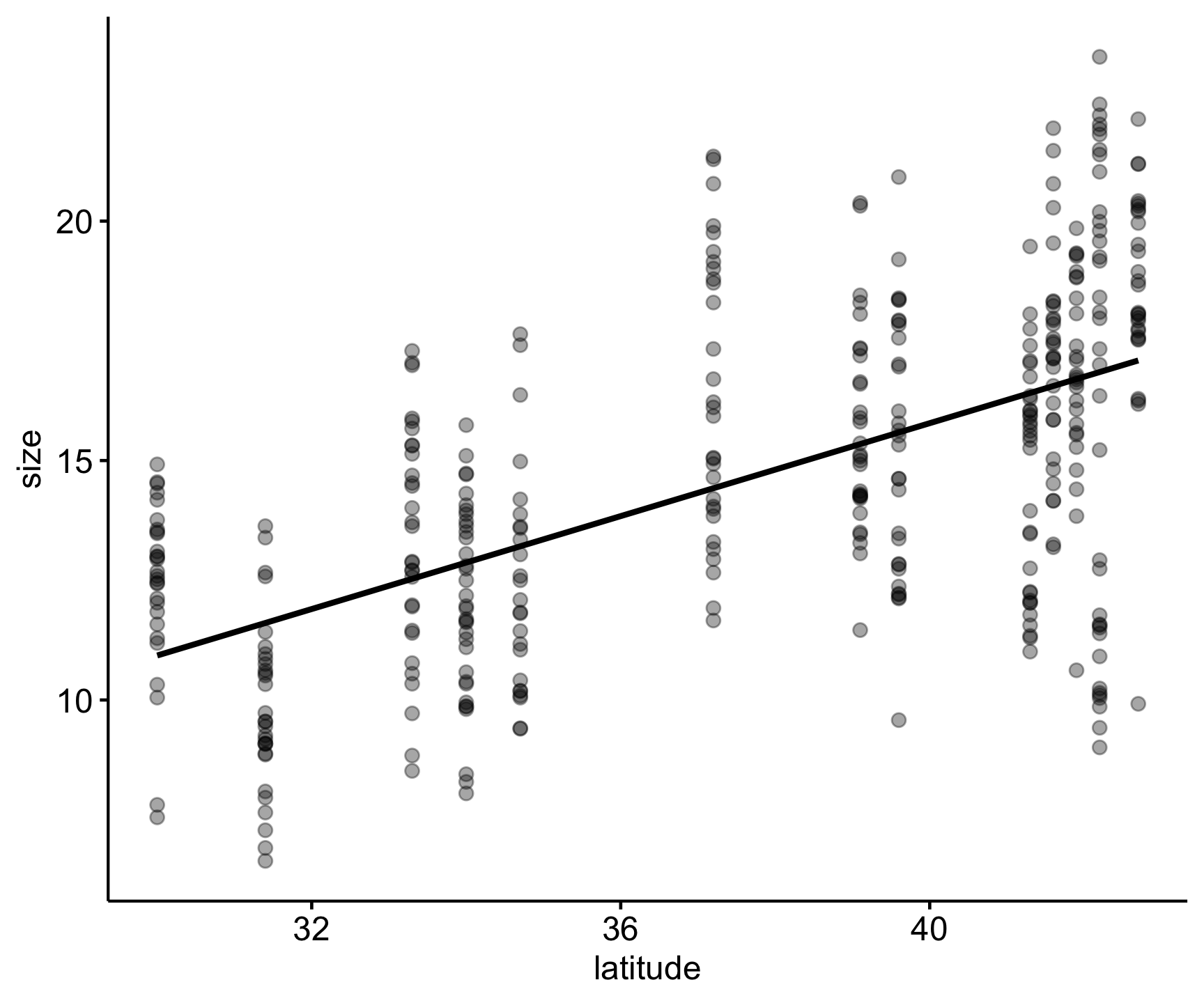

Predictions using a regression model

Now that we fit this model, we can use it to predict crab size at different latitudes with predict(). For example, let’s predict carapace width at a latitudes of 32, 36, and 38 degrees. Note that we need to create these values as a new data frame with the same column name used in the data that the model was built from.

Code

new_lat <- data.frame(latitude = c(32, 36, 38))

broom::augment(pie_lm, newdata = new_lat)

# A tibble: 3 × 2
  latitude .fitted
     <dbl>   <dbl>
1       32    11.9
2       36    13.8
3       38    14.8

Multiple Linear Regression

Say we want to model the effect of more than one predictor on crab size. In the data we also have continuous variables for air temperature and water temperature. Let’s model the effect of latitude, air and water temperature on carapace width.

Running a multiple linear regression is very similar to the simple linear regression, but now we specify our multiple predictor variables by adding them together with a + sign like this:

Code

pie_mlm <- lm(size ~ latitude + air_temp + water_temp, data = pie_crab)

summary(pie_mlm)


Call:
lm(formula = size ~ latitude + air_temp + water_temp, data = pie_crab)

Residuals:
    Min      1Q  Median      3Q     Max 
-8.7099 -1.7195 -0.0602  1.7823  7.7271 

Coefficients:
            Estimate Std. Error t value Pr(>|t|)    
(Intercept)  77.7460    17.3477   4.482 9.76e-06 ***
latitude     -1.0587     0.3174  -3.336 0.000933 ***
air_temp     -2.4041     0.3844  -6.255 1.05e-09 ***
water_temp    0.7563     0.1465   5.162 3.92e-07 ***
---
Signif. codes:  0 '***' 0.001 '**' 0.01 '*' 0.05 '.' 0.1 ' ' 1

Residual standard error: 2.677 on 388 degrees of freedom
Multiple R-squared:  0.4206,    Adjusted R-squared:  0.4161 
F-statistic:  93.9 on 3 and 388 DF,  p-value: < 2.2e-16

These results show an overall p-value for the model, indicating a significant impact of the combination of predictors on crab size, and individual p-values for the effect of each individual predictor on crab size.

Note however that with multiple regression, one of the assumptions is that there is no correlation between the predictor variables. We can test for correlations among more than two variables with the cor() function. Lets test for correlation between our three predictors:

Code

pie_crab |> 
  dplyr::select(latitude, air_temp, water_temp) |> 
  cor()

             latitude   air_temp water_temp
latitude    1.0000000 -0.9949715 -0.9571738
air_temp   -0.9949715  1.0000000  0.9632287
water_temp -0.9571738  0.9632287  1.0000000

It is usually good practice to remove variables from a multiple linear regression that have a correlation coefficient greater than 0.7/-0.7. These are all highly correlated (with coefficients near 1/-1), therefore they are not the best set of predictors to use for a multiple linear regression in combination. Highly correlated variables have nearly the same ability to predict the outcome (e.g., they do not bring additional information; they bring redundant information) and increase the complexity of the model and therefore the risk of errors.

In your assignment, you will perform a multiple linear regression using variables that are less correlated.

Exercises: Part 2

After completing the ANOVA test (and post-hoc Tukey’s HSD) above to test for significant differences in crab size among 3 different sites: 1) Create a boxplot showing the carapace width for each site where sites are ordered by latitude and 2) report the findings of the statistical test as you would in a scientific paper. Include both the code to create the boxplot and an image of the figure. (10 pts.)
Conduct a simple linear regression for the effect of water_temp_sd (a measure reflecting annual variation in water temperature) on carapace width. Report your findings (include code and a sentence reporting the results) AND create a plot with a line of best fit. Include both the code to create the plot and an image of the figure. (10 pts).
Conduct a multiple linear regression for the effects of latitude, air_temp_sd, and water_temp_sd on carapace width. First check for correlations among the three predictor variables (and report the correlation table) and second report your findings from the multiple linear regression (code and a sentence reporting the results). (10 pts.)

Acknowledgements

Thanks to the developers of lterdatasampler for providing the data set and vignettes that helped guide the creation of this lesson plan.

Citations

Johnson, D. 2019. Fiddler crab body size in salt marshes from Florida to Massachusetts, USA at PIE and VCR LTER and NOAA NERR sites during summer 2016. ver 1. Environmental Data Initiative. https://doi.org/10.6073/pasta/4c27d2e778d3325d3830a5142e3839bb (Accessed 2021-05-27).
Johnson DS, Crowley C, Longmire K, Nelson J, Williams B, Wittyngham S. The fiddler crab, Minuca pugnax, follows Bergmann’s rule. Ecol Evol. 2019;00:1–9. https://doi.org/10.1002/ece3.5883

Data Source: Gregory, S.V. and I. Arismendi. 2020. Aquatic Vertebrate Population Study in Mack Creek, Andrews Experimental Forest, 1987 to present ver 14. Environmental Data Initiative. https://doi.org/10.6073/pasta/7c78d662e847cdbe33584add8f809165

Kaylor, M.J. and D.R. Warren. 2017. Linking riparian shade and the legacies of forest management to fish and vertebrate biomass in forested streams. Ecosphere 8(6). https://doi.org/10.1002/ecs2.1845