Lab 8: Machine Learning

The Whole Game Plan

The Whole Game Plan

In Unit 3, we have learned a lot about the Machine Learning process. We have learned about feature engineering, resampling, the different types of machine learning goals, the different types of models (and R engines), and how to evaluate the performance and tune a final model.

We have also learned about the importance of data splitting and how to use the tidymodels package to create a machine learning pipeline.

In this lab, we will put all of this knowledge together to create a complete machine learning pipeline for a regression problem.

Lab Set Up

1. Open your existing lab 6 project
2. Create a new Quarto document called hyperparameter-tuning.qmd in the project folder (next to your lab6.qmd).
3. Start with the lab!

Libraries

Lets return to the CAMELS dataset we have been working with in Lab 6. We will use this dataset to predict the q_mean variable using the other variables in the dataset.

• Load the tidyverse and tidymodels packages

Data Import/Tidy/Transform

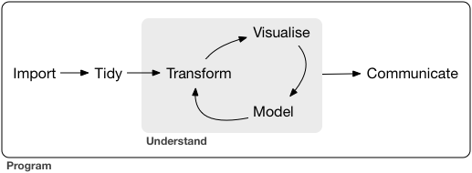
Your first job is to read in the data and clean it. This is the first step in any data science process in order to prepare the data for modeling and or analysis.

• Read in the data using map, read_delim() and powerjoin::power_full_join(). If you need a refresher on this please refer to lab 6.

• Clean the data using dplyr, EDA (skimr, visdat, ggpubr), and other means to ensure it is in a good form for modeling.

• At the end of this lab you will need to make a map of your predictions so be sure not to loose the gauge_lat and gauge_lon columns.

Data Spliting

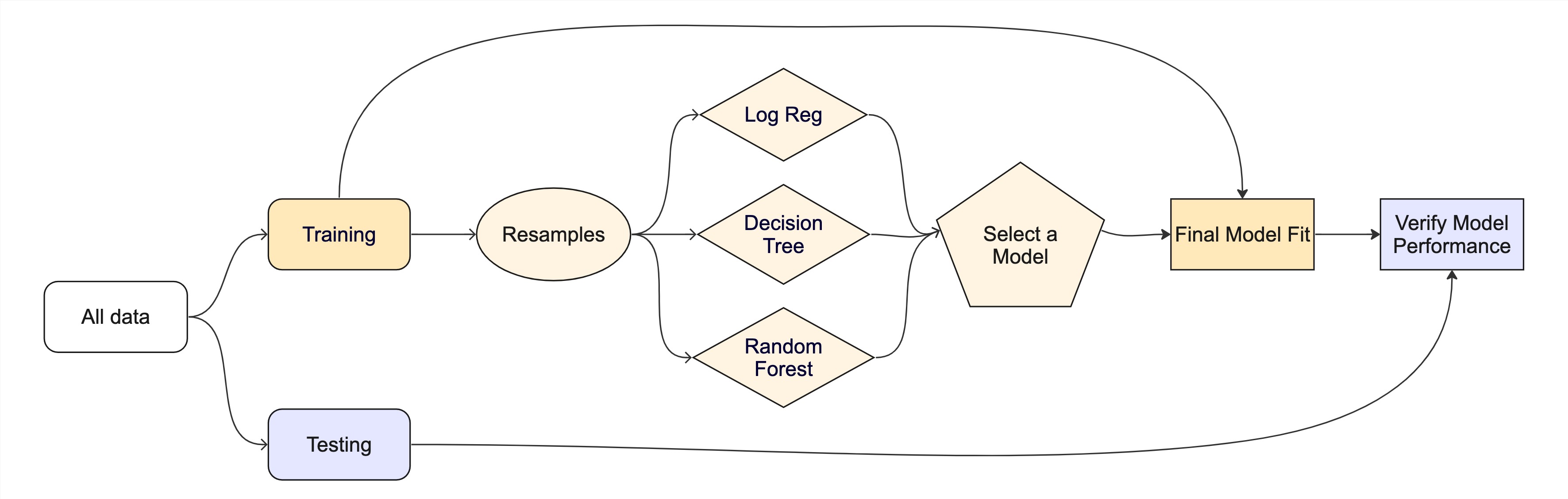
Now that you have your data cleaned and in a good form, you are ready to split the data into a training and testing set.

• Be sure to set a seed to ensure the random process is reproducable.
• Use the initial_split() function from the rsample package to split the data. Use 80% of the data for training and 20% for testing.
• Use the training() and testing() functions from the rsample package to extract the training and testing data.frames.

Feature Engineering

Not all data - even cleaned data - is primed for model input. In this class we have looked at recipes as a way of defining a preprocessor for our modeling efforts. Recipes are a way of defining a set of steps to be applied to the data anytime it is used. They require a formula and incremental steps to transform a dataset.

• Use the recipe() function from the recipes package to create a recipe object. The formula should be based on how you want to predict q_mean and the data should be the training data. Remember to apply any data transformations you deem needed, and be sure not to transform the outcome variable directly in the recipe.

• You should not use gauge_lat and gauge_lon in the recipe as predictors. You can use the step_rm() function to remove them from the recipe while ensureing they persist in any data passed throuhg fit_*.

Resampling and Model Testing

Your training data is now ready to be used for model training and you have a preprocessor that you can iterate over.

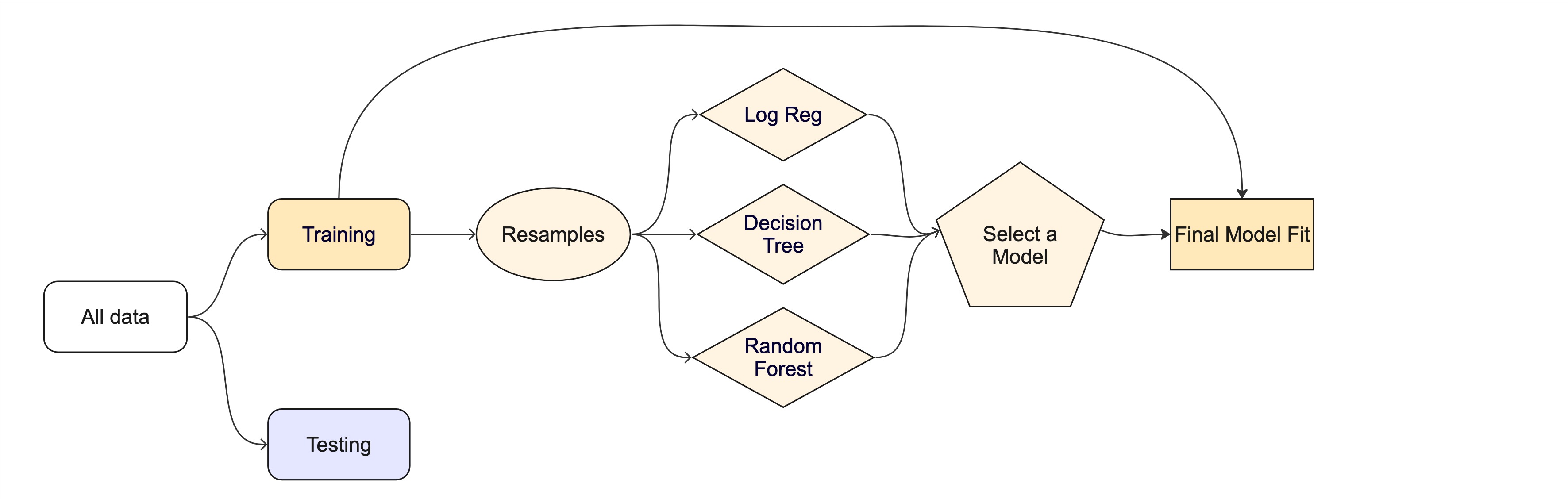
1. Build resamples

• The first step is to resample the data using the vfold_cv() function to generate 10 k-fold samples for cross-validation. Remember Cross Validation is critical for model testing and evaluation.

2. Build 3 Candidate Models

You will also define a set of models to test. A model is defined by a specification, an engine, and a mode. The specification defines the type of model and the engine defines the implementation of the model. In class we learned about a few classes of models including

 - Linear models
 - Logistic regression
 - Decision trees
 - Random forests
 - Boosted trees
 - Support vector machines
 - Neural networks

• Define 3 models that you feel have the best chance of performing well on the data. You can use any of the models we have learned about in class. You can also use any of the engines we have learned about in class. The below image is illustrative, not dictating the models to choose.

3. Test the models

With your defined set of models, k-folds samples, and recipe you are ready to test the models.

• Use the workflow_set() function to test your three models against the recipe. You will use the workflow_map() function to map the models to the recipe and resamples.

• Once complete, use autoplot to visualize the results of the workflow set.

4. Model Selection

• Based on the visualized metrics, select a model that you think best performs. Describe the reason for your choice using the metrics.

• Describe the model you selected. What is the model type, engine, and mode. Why do you think it is performing well for this problem?

Model Tuning

OK! Now you have selected a base model to use. Now we are interested in tuning it to extract the maximum performance that we can from it. Remember that all models have hyderparameters that are used to refine the underlying algorithm (specification)

1. Build a model for your chosen specification.

Be sure to set the mode and engine as you did above but this time specify at least 2 hyperparameters to tune using the tune() function. These are set in the model specification and options can be found in the documentation for the model you are using.

• Define a tunable model

2. Create a workflow

Now create a workflow object for this tune-able model and the recipe you created above.

• Create a workflow object using the workflow() that adds your recipe and tunable model.

3. Check The Tunable Values / Ranges

In the above step, you created a workflow based on a model that has at least 2 tunable hyper parameters. Remember tune() is aware of the tunable parameters in the model specification and provides some basic defaults to tune across. We want to see what the range of those are!

To do this, we can use the extract_parameter_set_dials()to return a list of the tunable parameters and their ranges. The output of this function is a data.frame.

• Use the extract_parameter_set_dials(YOUR MODEL WORKFLOW) and save it to an object named dials. Check the dials$object slot to see the tunable parameters and their ranges.

• Optionally, you could update these default ranges using update. But for this lab, we will stick with the defaults.

4. Define the Search Space

OK, we now know the viable range of the hyperparameters we want to tune. The full range of these values is the complete search space in which the best options could live. Remember, there are two ways for our computer to search for the best combination:

1. Grid Search: This is a brute force approach that tests a predefined set of combinations. If elected as the search process, we need to specify how the set of combinations is chosen. This can be versions of evenly spaced (regular), random, or space filling curve/design (SFC/SFD).
2. Iterative: This is a more efficient approach that uses a set of algorithms to search the space. This is often more efficient than grid search, but can be less thorough.

For this lab, lets use a grid search based on a “Latin Hypercube” SFD method. We can specify this by passing our above dials object to the grid_latin_hypercube() function. The only thing we need to specify is the size of the grid we want to evaluate. The larger the size, the more thorough the search, but the longer your computer will take. Lets set the size to 20 for this lab and save the outputs to an object called my.grid.

• Create a SFD Grid Object with 25 predefined combinations.

5. Tune the Model

OK! You now have a tunable model workflow (wf_tune), a set of k-fold resamples to test over (folds), and a grid of hyperparameters to search (grid). Now we can use the tune_grid() function to search the grid and evaluate the model performance using the code below. In this example, we are doing 2 additional things. Setting a set of metrics to compute and saving the predictions to a output tibble.

• Run the below code making any changes your need based on how you named your objects.
• Run autoplot() on the model_params object to visualize the results of the tuning process.
• Describe what you see!

model_params <-  tune_grid(
    wf_tune,
    resamples = folds,
    grid = my.grid,
    metrics = metric_set(rmse, rsq, mae),
    control = control_grid(save_pred = TRUE)
  )

autoplot(model_params)

6. Check the skill of the tuned model

Now that you have tuned the model under many combinations of hyperparameters, you can check the skill using the collect_metrics() function. This will return a tibble with the metrics for each combination of hyperparameters.

• Use the collect_metrics() function to check the skill of the tuned model. Describe what you see, remember dplyr functions like arrange, slice_*, and filter will work on this tibble.

You can also use the show_best() function to show the best performing model based on a metric of your choice. For example, if you want to see the best performing model based on the RMSE metric, you can use the following code:

• Use the show_best() function to show the best performing model based on Mean Absolute Error.

• Please interpret the results of the first row of show_best(). What do you see? What hyperparameter set is best for this model, based on MAE?

A short cut for show_best(..., n = 1) is to use select_best(). This will return the best performing hyperparameter set based on the metric you choose.

• Use the select_best() function to save the best performing hyperparameter set to an object called hp_best.

7. Finalize your model

Fantastic, you now have a workflow and a idealized set of hyperparameters to use for your model. Now we can inject the hyperparameters into the workflow using the finalize_workflow() function. This will create a new workflow object that is no longer dependent on tune() attributes, but rather the finalized hyperparameters. This is a new workflow object that is ready to be used for final model fitting.

• Run finalize_workflow() based on your workflow and best hyperparmater set to create a final workflow object.

Final Model Verification

The show_best(), select_best(), and collect_metrics() functions are all great, but they are only implemented on the resampled iterations of the training data. Remember, applications over just the training data can often be misleading. We need to check the final model on the test data to see how it performs.

Here, we can leverage a short cut in tidymodels to fit the final model to the test data. This is done using the last_fit() function. The last_fit() function will take the finalized workflow, and the full split data object (containing both the training and testing data) and fit it to the training data and validate it on the testing data.

• Use last_fit() to fit the finalized workflow the original split object (output of initial_split()). This will fit the model to the training data and validate it on the testing data.

With the final model fit, we can now check the performance of the model on the test data in our two standard ways!

• Use the collect_metrics() function to check the performance of the final model on the test data. This will return a tibble with the metrics for the final model.

• Interpret these results. How does the final model perform on the test data? Is it better or worse than the training data? Use your knowledge of the regression based metrics to describe the results.

• Use the collect_predictions() function to check the predictions of the final model on the test data. This will return a tibble with the predictions for the final model.

• Use the output of this to create a scatter plot of the predicted values vs the actual values. Use the ggplot2 package to create the plot. This plot should include (1) geom_smooth(method = “lm”) to add the linear fit of predictions and truth (2) geom_abline() to add a 1:1 line (3) nice colors via scale_color_* and (4) accurate labels.

Building a Map!

As a last step, you want to map your predictions across CONUS. Return to the ggplot examples in Lab 6 to refresh your memory on building a map with a defined color pallete.

To build your final prediction, you can use fit() to fit the finalized workflow to the full, cleaned data (prior to splitting). This will return a fitted model object that can be used to make predictions on new data.

• This full fit can be passed to the augment() function to make predictions on the full, cleaned data. This will return a tibble with the predictions for the full data.

• Use the mutate() function to calculate the residuals of the predictions. The residuals are the difference between the predicted values and the actual values squared.

• Use ggplot2 to create a map of the predictions.

• Use ggplot2 to create a map of the residuals.

• Use patchwork to combine the two maps into one figure.

Summary

And that’s it! You have implemented a complete, robust, and well tuned machine learning pipeline. You have learned how to read in data, clean it, split it, create a recipe, resample it, test models, tune models, and finally validate the model on the test data. This is NOT an insignificant amount of work and knowledge and I hope you are proud of how far you have come in this class.

Rubric

Task	Subtask	(Sub)Points
Data Import/Tidy/Transform		20
	Library Loading	5
	Data Ingest	5
	Data Cleaning	10
Data Spiting		10
	Initial Split	5
	Testing/Training	5
Feature Engineering		10
	Proper Recipe	10
Data Resampling and Model Testing		25
	Cross Validation Dataset (k-folds)	5
	Define Three Regression Models	10
	Workflow Set/Map/Autoplot	5
	Model Selection with Justification	5
Model Tuning		25
	Tunable model setup	5
	Tunable workflow defined	5
	Description of dial ranges	5
	Defined Search Space	5
	Executed Tune Grid	5
Check the skill of the tuned model		10
	Collect Metrics/Show Best/Describe in Plain Language	10
Finalize your model		5
	Finalize Workflow	5
Final Model Verification		25
	Implement the last fit	5
	Interpret Metrics	10
	Plot Predictions	10
Final Figure		20
	Augment Data & Calculate Residuals	5
	Map Predicted Q and Residuals	15
Submission		10
	Working URL	10

Total: 150

Submission

Once you have completed the above steps, you can submit your lab for grading. The lab should be submitted as a URL to your deployed repo page. The repo should contain the qmd file with all the code, data, and output used in the lab.