Lecture 19

Evaluation & Tuning

Recaping Day 1 - 4

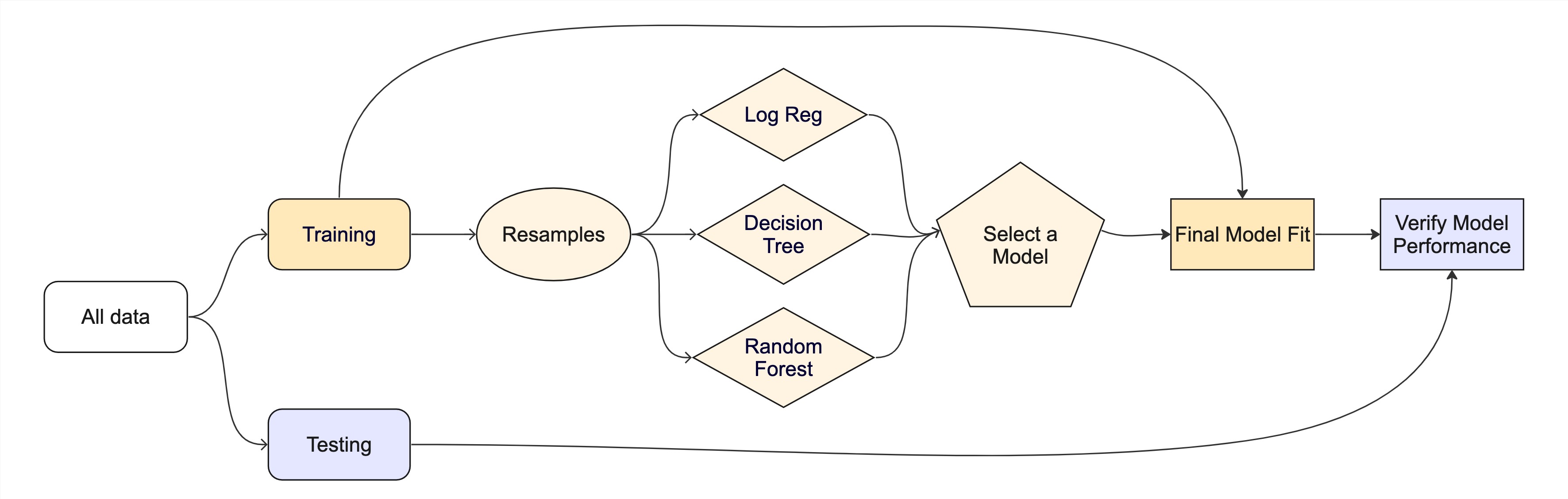
library(tidymodels)
library(forested)

# Set a seed
set.seed(123)

# IntitalizeInitialize Split
forested_split <- initial_split(forested, prop = 0.8)
forested_train <- training(forested_split)
forested_test  <- testing(forested_split)

# Build Resamples
forested_folds <- vfold_cv(forested_train, v = 10)

# Set a model specification with mode (default engine)
dt_mod         <- decision_tree(cost_complexity = 0.0001, mode = "classification")

# Bare bones workflow & fit
forested_wflow <- workflow(forested ~ ., dt_mod)
forested_fit   <- fit(forested_wflow, forested_train)

# Extracting Predictions:
augment(forested_fit, new_data = forested_train)
#> # A tibble: 5,685 × 22
#>    .pred_class .pred_Yes .pred_No forested  year elevation eastness northness
#>    <fct>           <dbl>    <dbl> <fct>    <dbl>     <dbl>    <dbl>     <dbl>
#>  1 No             0.0114   0.989  No        2016       464       -5       -99
#>  2 Yes            0.636    0.364  Yes       2016       166       92        37
#>  3 No             0.0114   0.989  No        2016       644      -85       -52
#>  4 Yes            0.977    0.0226 Yes       2014      1285        4        99
#>  5 Yes            0.977    0.0226 Yes       2013       822       87        48
#>  6 Yes            0.808    0.192  Yes       2017         3        6       -99
#>  7 Yes            0.977    0.0226 Yes       2014      2041      -95        28
#>  8 Yes            0.977    0.0226 Yes       2015      1009       -8        99
#>  9 No             0.0114   0.989  No        2017       436      -98        19
#> 10 No             0.0114   0.989  No        2018       775       63        76
#> # ℹ 5,675 more rows
#> # ℹ 14 more variables: roughness <dbl>, tree_no_tree <fct>, dew_temp <dbl>,
#> #   precip_annual <dbl>, temp_annual_mean <dbl>, temp_annual_min <dbl>,
#> #   temp_annual_max <dbl>, temp_january_min <dbl>, vapor_min <dbl>,
#> #   vapor_max <dbl>, canopy_cover <dbl>, lon <dbl>, lat <dbl>, land_type <fct>

Evaluation

So far we have used metrics and collect_metrics to evaluate and compare models
The default metrics for classification problems are: accuracy, brier_score, roc_auc
- All classification metrics stem from the classic confusion matrix

The default metrics for regression problems are: rsq, rmse, mae
- The majority of these are measures of correlation and residual error

Classification:

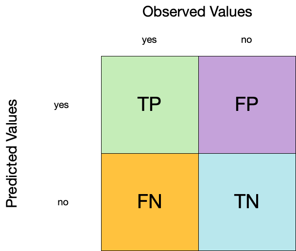
Confusion matrix

A confusion matrix is a table that describes the performance of a classification model on a set of data for which the true values are known.
It counts the number of accurate and false predictions, separated by the truth state

augment(forested_fit, new_data = forested_train) |>
  conf_mat(truth = forested, estimate = .pred_class)
#>           Truth
#> Prediction  Yes   No
#>        Yes 2991  176
#>        No   144 2374

What to do with a confusion matrix

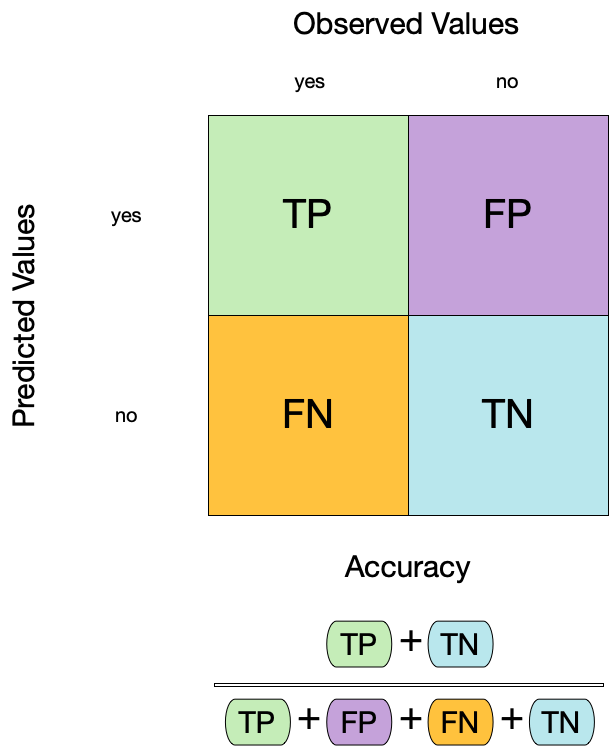
1. Accuracy

Accuracy is the proportion of true results (both true positives and true negatives) among the total number of cases examined.
It is a measure of the correctness of the model’s predictions.
It is the most common metric used to evaluate classification models.

augment(forested_fit, new_data = forested_train) |>
  accuracy(truth = forested, estimate = .pred_class)
#> # A tibble: 1 × 3
#>   .metric  .estimator .estimate
#>   <chr>    <chr>          <dbl>
#> 1 accuracy binary         0.944

2. Sensitivity

Sensitivity is the proportion of true positives to the sum of true positives and false negatives.
It is useful for identifying the presence of a condition.
It is also known as the true positive rate, recall, or probability of detection.

augment(forested_fit, new_data = forested_train) |>
  sensitivity(truth = forested, estimate = .pred_class)
#> # A tibble: 1 × 3
#>   .metric     .estimator .estimate
#>   <chr>       <chr>          <dbl>
#> 1 sensitivity binary         0.954

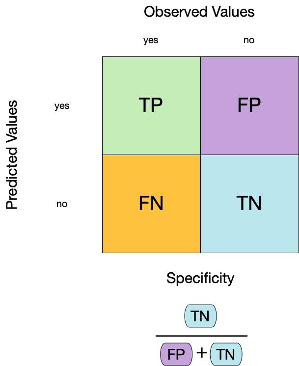
3. Specificity

Specificity is the proportion of true negatives to the sum of true negatives and false positives.
It is useful for identifying the absence of a condition.
It is also known as the true negative rate, and is the complement of sensitivity.

augment(forested_fit, new_data = forested_train) |>
  sensitivity(truth = forested, estimate = .pred_class)
#> # A tibble: 1 × 3
#>   .metric     .estimator .estimate
#>   <chr>       <chr>          <dbl>
#> 1 sensitivity binary         0.954

augment(forested_fit, new_data = forested_train) |>
  specificity(truth = forested, estimate = .pred_class)
#> # A tibble: 1 × 3
#>   .metric     .estimator .estimate
#>   <chr>       <chr>          <dbl>
#> 1 specificity binary         0.931

Two class data

These metrics assume that we know the threshold for converting “soft” probability predictions into “hard” class predictions.

For example, if the predicted probability of a tree is 0.7, we might say that the model predicts “Tree” for that observation.
If the predicted probability of a tree is 0.4, we might say that the model predicts “No tree” for that observation.
The threshold is the value that separates the two classes.
The default threshold is 0.5, but this can be changed.

Is a 50% threshold good?

What happens if we say that we need to be 80% sure to declare an event?

sensitivity ⬇️, specificity ⬆️

What happens for a 20% threshold?

sensitivity ⬆️, specificity ⬇️

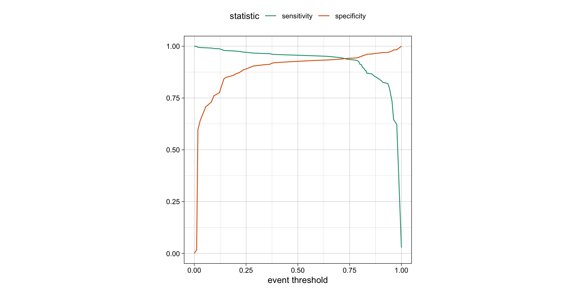
Varying the threshold

The threshold can be varied to see how it affects the sensitivity and specificity of the model.
This is done by plotting the sensitivity and specificity against the threshold.
The threshold is varied from 0 to 1, and the sensitivity and specificity are calculated at each threshold.
The plot shows the trade-off between sensitivity and specificity at different thresholds.
The threshold can be chosen based on the desired balance between sensitivity and specificity.

ROC curves

For an ROC (receiver operator characteristic) curve, we plot

the false positive rate (1 - specificity) on the x-axis
the true positive rate (sensitivity) on the y-axis

with sensitivity and specificity calculated at all possible thresholds.

ROC curves

The ROC AUC is the probability that a randomly chosen positive instance is ranked higher than a randomly chosen negative instance.

The ROC AUC is a measure of how well the model separates the two classes.
The ROC AUC is a number between 0 and 1.
ROC AUC = 1 💯
- perfect classification
ROC AUC = 0.5 😐
- random guessing
ROC AUC < 0.5 😱
- worse than random guessing

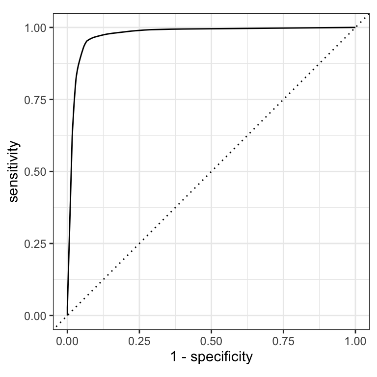
ROC curves

(A ROC AUC of 0.7-0.8 is considered acceptable, 0.8-0.9 is good, and >0.9 is excellent.)

# Assumes _first_ factor level is event; there are options to change that
augment(forested_fit, new_data = forested_train) |>  
  roc_curve(truth = forested, .pred_Yes)  |> 
  dplyr::slice(1, 20, 50)
#> # A tibble: 3 × 3
#>   .threshold specificity sensitivity
#>        <dbl>       <dbl>       <dbl>
#> 1   -Inf           0           1    
#> 2      0.235       0.885       0.972
#> 3      0.909       0.969       0.826

augment(forested_fit, new_data = forested_train) |>  
  roc_auc(truth = forested, .pred_Yes)
#> # A tibble: 1 × 3
#>   .metric .estimator .estimate
#>   <chr>   <chr>          <dbl>
#> 1 roc_auc binary         0.975

Brier score

The Brier score is a measure of how well the predicted probabilities of an event match the actual outcomes.
It is the mean squared difference between predicted probabilities and actual outcomes.
The Brier score is a number between 0 and 1.
The Brier score is analogous to the mean squared error in regression models:
Brier = 1 😱
- predicted probabilities are completely wrong
Brier = 0.5 😐
- bad
Brier < 0.25
- acceptable
Brier = 0 💯
- predicted probabilities are perfect

\[ Brier_{class} = \frac{1}{N}\sum_{i=1}^N\sum_{k=1}^C (y_{ik} - \hat{p}_{ik})^2 \]

Brier score

augment(forested_fit, new_data = forested_train) |>  
  brier_class(truth = forested, .pred_Yes) 
#> # A tibble: 1 × 3
#>   .metric     .estimator .estimate
#>   <chr>       <chr>          <dbl>
#> 1 brier_class binary        0.0469

Separation vs calibration

The ROC captures separation. - The ROC curve shows the trade-off between sensitivity and specificity at different thresholds.

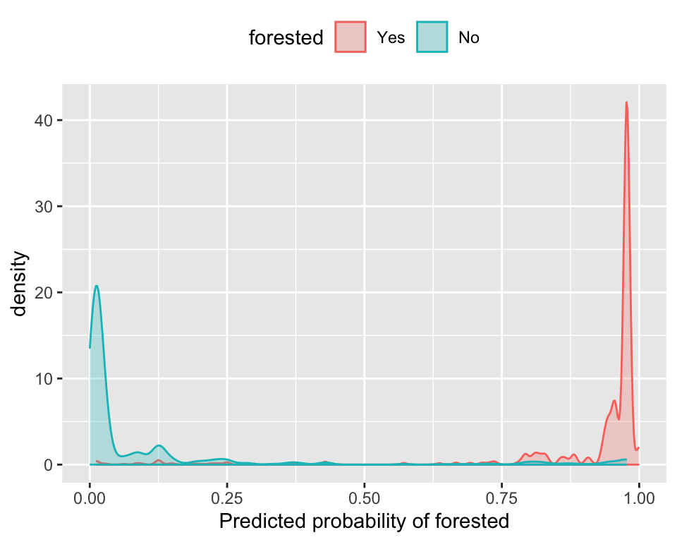
The Brier score captures calibration. - The Brier score is a measure of how well the predicted probabilities of an event match the actual outcomes.

Good separation: the densities don’t overlap.
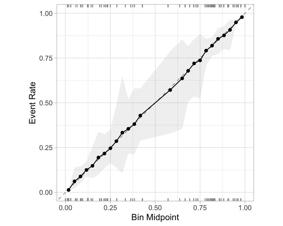
Good calibration: the calibration line follows the diagonal.

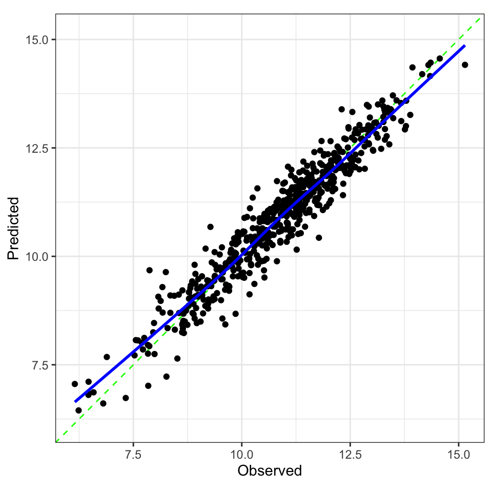
Calibration plot: We bin observations according to predicted probability. In the bin for 20%-30% predicted prob, we should see an event rate of ~25% if the model is well-calibrated.

Regression

R-squared (\(R^2\))

Measures how well the model explains the variance in the data.
Formula:

\[ R^2 = 1 - \frac{SS_{res}}{SS_{tot}} \] where:
- \(SS_{res}\) is the sum of squared residuals.

\(SS_{tot}\) is the total sum of squares.
Values range from \(-\infty\) to 1.
- 1: Perfect fit
- 0: No improvement over mean prediction
- Negative: Worse than just using the mean

Root Mean Squared Error (RMSE)

Measures the model’s prediction error in the same unit as the dependent variable.
Formula:

\[ RMSE = \sqrt{\frac{1}{n} \sum_{i=1}^{n} (y_i - \hat{y}_i)^2} \]

where: - \(y_i\) is the actual value. - \(\hat{y}_i\) is the predicted value.

Penalizes large errors more than MAE.
Lower RMSE indicates better model performance.

Mean Absolute Error (MAE)

Measures average absolute errors between predictions and actual values.
Formula:

\[ MAE = \frac{1}{n} \sum_{i=1}^{n} |y_i - \hat{y}_i| \]

Less sensitive to outliers than RMSE.
Lower MAE indicates better model performance.

Comparing Metrics

Metric	Interpretation	Sensitivity to Outliers
\(R^2\)	Variance explained	Moderate
RMSE	Penalizes large errors more	High
MAE	Average error size	Low

Choosing the Right Metric

Use \(R^2\) to assess model fit and explainability.
Use RMSE if large errors are especially undesirable.
Use MAE for a more interpretable, robust metric.

Metrics Selection model performance

We can use metric_set() to combine multiple calculations into one

forested_metrics <- metric_set(accuracy, specificity, sensitivity)

augment(forested_fit, new_data = forested_train) |>
  forested_metrics(truth = forested, estimate = .pred_class)
#> # A tibble: 3 × 3
#>   .metric     .estimator .estimate
#>   <chr>       <chr>          <dbl>
#> 1 accuracy    binary         0.944
#> 2 specificity binary         0.931
#> 3 sensitivity binary         0.954

Metrics and metric sets work with grouped data frames!

augment(forested_fit, new_data = forested_train) |>
  group_by(tree_no_tree) |>
  accuracy(truth = forested, estimate = .pred_class)
#> # A tibble: 2 × 4
#>   tree_no_tree .metric  .estimator .estimate
#>   <fct>        <chr>    <chr>          <dbl>
#> 1 Tree         accuracy binary         0.946
#> 2 No tree      accuracy binary         0.941

augment(forested_fit, new_data = forested_train) |>
  group_by(tree_no_tree) |>
  specificity(truth = forested, estimate = .pred_class)
#> # A tibble: 2 × 4
#>   tree_no_tree .metric     .estimator .estimate
#>   <fct>        <chr>       <chr>          <dbl>
#> 1 Tree         specificity binary         0.582
#> 2 No tree      specificity binary         0.974

Note

The specificity for "Tree" is a good bit lower than it is for "No tree".

So, when this index classifies the plot as having a tree, the model does not do well at correctly identifying the plot as non-forested when it is indeed non-forested.

Recap

Previously - Setup

library(tidyverse)
# Ingest Data
# URLs for COVID-19 case data and census population data
covid_url <- 'https://raw.githubusercontent.com/nytimes/covid-19-data/master/us-states.csv'
pop_url <-  '/Users/mikejohnson/Downloads/co-est2023-alldata.csv'
#pop_url   <- 'https://www2.census.gov/programs-surveys/popest/datasets/2020-2023/counties/totals/co-est2023-alldata.csv'

# Clean Census Data
census = readr::read_csv(pop_url)  |> 
  filter(COUNTY == "000") |>  # Filter for state-level data only
  mutate(fips = STATE) |>      # Create a new FIPS column for merging
  select(fips, contains("2021"))  # Select relevant columns for 2021 data

# Process COVID-19 Data
state_data <-  readr::read_csv(covid_url) |> 
  group_by(fips) |> 
  mutate(
    new_cases  = pmax(0, cases  - dplyr::lag(cases)),   # Compute new cases, ensuring no negative values
    new_deaths = pmax(0, deaths - dplyr::lag(deaths))  # Compute new deaths, ensuring no negative values
  ) |> 
  ungroup() |> 
  left_join(census, by = "fips") |>  # Merge with census data
  mutate(
    m = month(date), y = year(date),
    season = case_when(   # Define seasons based on month
      m %in% 3:5 ~ "Spring",
      m %in% 6:8 ~ "Summer",
      m %in% 9:11 ~ "Fall",
      m %in% c(12, 1, 2) ~ "Winter"
    )
  ) |> 
  group_by(state, y, season) |> 
  mutate(
    season_cases  = sum(new_cases, na.rm = TRUE),  # Aggregate seasonal cases
    season_deaths = sum(new_deaths, na.rm = TRUE)  # Aggregate seasonal deaths
  )  |> 
  distinct(state, y, season, .keep_all = TRUE) |>  # Keep only distinct rows by state, year, season
  ungroup() |> 
  select(state, contains('season'), y, POPESTIMATE2021, BIRTHS2021, DEATHS2021) |>  # Select relevant columns
  drop_na() |>  # Remove rows with missing values
  mutate(logC = log(season_cases +1))  # Log-transform case numbers for modeling

Previously - Data Usage

set.seed(4028)
split <- initial_split(state_data, prop = 0.8, strata = season)  # 80/20 train-test split
train <- training(split)  # Training set
test <- testing(split)  # Test set

set.seed(3045)
folds <- vfold_cv(train, v = 10)  # 10-fold cross-validation

Previously - Feature engineering

rec = recipe(logC ~ . , data = train) |> 
  step_rm(state, season_cases) |>  # Remove non-predictive columns
  step_dummy(all_nominal()) |>  # Convert categorical variables to dummy variables
  step_scale(all_numeric_predictors()) |>  # Scale numeric predictors
  step_center(all_numeric_predictors())

Optimizing Models via Tuning Hyperparameter

Tuning parameters

Some model or preprocessing parameters cannot be estimated directly from the data.
Try different values and measure their performance.

Find good values for these parameters.

Once the value(s) of the parameter(s) are determined, a model can be finalized by fitting the model to the entire training set.

Tagging parameters for tuning

With tidymodels, you can mark the parameters that you want to optimize with a value of tune().

The function itself just returns… itself:

tune()
#> tune()

str(tune())
#>  language tune()

# optionally add a label
tune("Marker")
#> tune("Marker")

Boosted Trees

In last weeks live demo, a boosted tree proved most effective.

Boosted Trees are popular ensemble methods that build a sequence of tree models.

Each tree uses the results of the previous tree to better predict samples, especially those that have been poorly predicted.

Each tree in the ensemble is saved and new samples are predicted using a weighted average of the votes of each tree in the ensemble.

Boosted Tree Tuning Parameters

Some possible parameters:

mtry: The number of predictors randomly sampled at each split (in \([1, ncol(x)]\) or \((0, 1]\)).
trees: The number of trees (\([1, \infty]\), but usually up to thousands)
min_n: The number of samples needed to further split (\([1, n]\)).
learn_rate: The rate that each tree adapts from previous iterations (\((0, \infty]\), usual maximum is 0.1).
stop_iter: The number of iterations of boosting where no improvement was shown before stopping (\([1, trees]\))

Boosted Tree Tuning Parameters

b_mod <- 
  boost_tree(trees = tune(), learn_rate = tune()) |> 
  set_mode("regression") |> 
  set_engine("xgboost")

(b_wflow <- workflow(rec, b_mod))
#> ══ Workflow ════════════════════════════════════════════════════════════════════════════════════════════════════════════════════════════════════════════════════════════════════════════════════════════
#> Preprocessor: Recipe
#> Model: boost_tree()
#> 
#> ── Preprocessor ────────────────────────────────────────────────────────────────────────────────────────────────────────────────────────────────────────────────────────────────────────────────────────
#> 4 Recipe Steps
#> 
#> • step_rm()
#> • step_dummy()
#> • step_scale()
#> • step_center()
#> 
#> ── Model ───────────────────────────────────────────────────────────────────────────────────────────────────────────────────────────────────────────────────────────────────────────────────────────────
#> Boosted Tree Model Specification (regression)
#> 
#> Main Arguments:
#>   trees = tune()
#>   learn_rate = tune()
#> 
#> Computational engine: xgboost

Optimize tuning parameters

The main two strategies for optimization are:

Grid search 💠 which tests a pre-defined set of candidate values
Iterative search 🌀 which suggests/estimates new values of candidate parameters to evaluate

1. Grid search

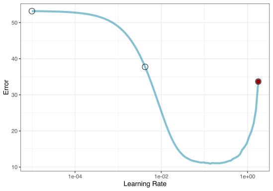
Most basic (but very effective) way to tune models
A small grid of points trying to minimize the error via learning rate:

1. Grid search

In reality we would probably sample the space more densely:

2. Iterative Search

We could start with a few points and search the space:

Grid Search Example

Parameters

The tidymodels framework provides pre-defined information on tuning parameters (such as their type, range, transformations, etc).
The extract_parameter_set_dials() function extracts these tuning parameters and the info.

Grids

Create your grid manually or automatically.
The grid_*() functions can make a grid.

Different types of grids

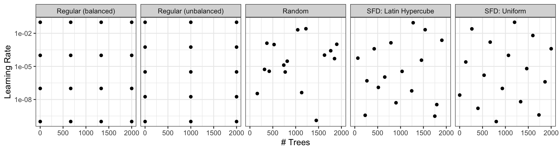
Space-filling designs (SFD) attempt to cover the parameter space without redundant candidates. We recommend these the most.

Create a grid

# Extac
(b_wflow |> 
  extract_parameter_set_dials())

# Individual functions: 
(trees())
(learn_rate())

A parameter set can be updated (e.g. to change the ranges).

Create a grid

The grid_*() functions create a grid of parameter values to evaluate.
The grid_space_filling() function creates a space-filling design (SFD) of parameter values to evaluate.
The grid_regular() function creates a regular grid of parameter values to evaluate.
The grid_random() function creates a random grid of parameter values to evaluate.
The grid_latin_hypercube() function creates a Latin hypercube design of parameter values to evaluate.
The grid_max_entropy() function creates a maximum entropy design of parameter values to evaluate.

Create a SFD curve

set.seed(12)

(grid <- 
  b_wflow |> 
  extract_parameter_set_dials() |> 
  grid_space_filling(size = 25))
#> # A tibble: 25 × 2
#>    trees learn_rate
#>    <int>      <dbl>
#>  1     1    0.0287 
#>  2    84    0.00536
#>  3   167    0.121  
#>  4   250    0.00162
#>  5   334    0.0140 
#>  6   417    0.0464 
#>  7   500    0.196  
#>  8   584    0.00422
#>  9   667    0.00127
#> 10   750    0.0178 
#> # ℹ 15 more rows

Create a regular grid

set.seed(12)

(grid <- 
  b_wflow |> 
  extract_parameter_set_dials() |> 
  grid_regular(levels = 4))
#> # A tibble: 16 × 2
#>    trees learn_rate
#>    <int>      <dbl>
#>  1     1    0.001  
#>  2   667    0.001  
#>  3  1333    0.001  
#>  4  2000    0.001  
#>  5     1    0.00681
#>  6   667    0.00681
#>  7  1333    0.00681
#>  8  2000    0.00681
#>  9     1    0.0464 
#> 10   667    0.0464 
#> 11  1333    0.0464 
#> 12  2000    0.0464 
#> 13     1    0.316  
#> 14   667    0.316  
#> 15  1333    0.316  
#> 16  2000    0.316

Update parameter ranges

b_param <- 
  b_wflow |> 
  extract_parameter_set_dials() |> 
  update(trees = trees(c(1L, 100L)),
         learn_rate = learn_rate(c(-5, -1)))

set.seed(712)
(grid <- 
  b_param |> 
  grid_space_filling(size = 25))
#> # A tibble: 25 × 2
#>    trees learn_rate
#>    <int>      <dbl>
#>  1     1  0.00215  
#>  2     5  0.000147 
#>  3     9  0.0215   
#>  4    13  0.0000215
#>  5    17  0.000681 
#>  6    21  0.00464  
#>  7    25  0.0464   
#>  8    29  0.0001   
#>  9    34  0.0000147
#> 10    38  0.001    
#> # ℹ 15 more rows

The results

grid |> 
  ggplot(aes(trees, learn_rate)) +
  geom_point(size = 4) +
  scale_y_log10()

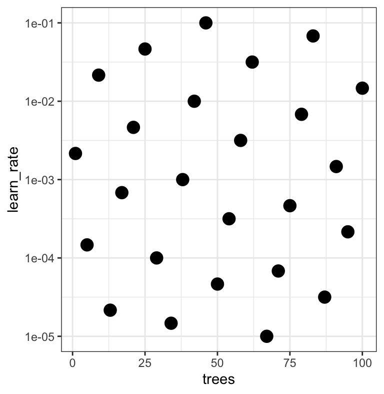
Note that the learning rates are uniform on the log-10 scale and this shows 2 of 4 dimensions.

Use the `tune_*()` functions to tune models

Choosing tuning parameters

Let’s take our previous model and tune more parameters:

b_mod <- 
  boost_tree(trees = tune(), learn_rate = tune(),  min_n = tune()) |> 
  set_mode("regression") |> 
  set_engine("xgboost")

b_wflow <- workflow(rec, b_mod)

# Update the feature hash ranges (log-2 units)
b_param <-
  b_wflow |>
  extract_parameter_set_dials() |>
  update(trees = trees(c(1L, 1000L)))

Grid Search

set.seed(9)
ctrl <- control_grid(save_pred = TRUE)

b_res <-
  b_wflow |>
  tune_grid(
    resamples = folds,
    grid = 25,
    # The options below are not required by default
    param_info = b_param, 
    control = ctrl,
    metrics = metric_set(mae)
  )

Grid Search

b_res 
#> # Tuning results
#> # 10-fold cross-validation 
#> # A tibble: 10 × 5
#>    splits           id     .metrics          .notes           .predictions        
#>    <list>           <chr>  <list>            <list>           <list>              
#>  1 <split [513/57]> Fold01 <tibble [25 × 7]> <tibble [0 × 3]> <tibble [1,425 × 7]>
#>  2 <split [513/57]> Fold02 <tibble [25 × 7]> <tibble [0 × 3]> <tibble [1,425 × 7]>
#>  3 <split [513/57]> Fold03 <tibble [25 × 7]> <tibble [0 × 3]> <tibble [1,425 × 7]>
#>  4 <split [513/57]> Fold04 <tibble [25 × 7]> <tibble [0 × 3]> <tibble [1,425 × 7]>
#>  5 <split [513/57]> Fold05 <tibble [25 × 7]> <tibble [0 × 3]> <tibble [1,425 × 7]>
#>  6 <split [513/57]> Fold06 <tibble [25 × 7]> <tibble [0 × 3]> <tibble [1,425 × 7]>
#>  7 <split [513/57]> Fold07 <tibble [25 × 7]> <tibble [0 × 3]> <tibble [1,425 × 7]>
#>  8 <split [513/57]> Fold08 <tibble [25 × 7]> <tibble [0 × 3]> <tibble [1,425 × 7]>
#>  9 <split [513/57]> Fold09 <tibble [25 × 7]> <tibble [0 × 3]> <tibble [1,425 × 7]>
#> 10 <split [513/57]> Fold10 <tibble [25 × 7]> <tibble [0 × 3]> <tibble [1,425 × 7]>

Grid results

autoplot(b_res)

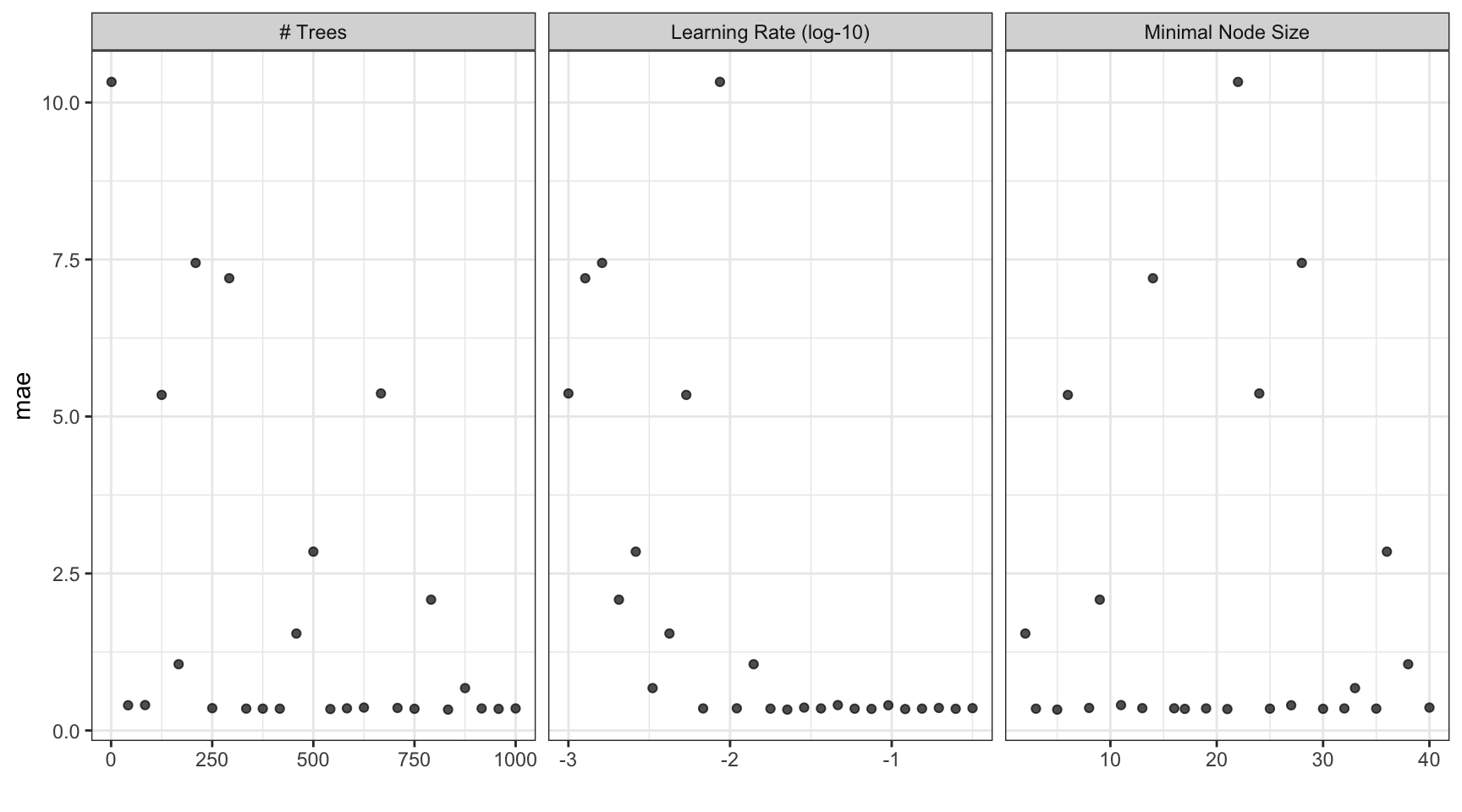
Tuning results

collect_metrics(b_res)
#> # A tibble: 25 × 9
#>    trees min_n learn_rate .metric .estimator  mean     n std_err .config              
#>    <int> <int>      <dbl> <chr>   <chr>      <dbl> <int>   <dbl> <chr>                
#>  1   458     2    0.00422 mae     standard   1.54     10  0.0259 Preprocessor1_Model01
#>  2   417     3    0.0590  mae     standard   0.347    10  0.0143 Preprocessor1_Model02
#>  3   833     5    0.0226  mae     standard   0.333    10  0.0133 Preprocessor1_Model03
#>  4   125     6    0.00536 mae     standard   5.34     10  0.0476 Preprocessor1_Model04
#>  5   708     8    0.196   mae     standard   0.359    10  0.0120 Preprocessor1_Model05
#>  6   791     9    0.00205 mae     standard   2.08     10  0.0300 Preprocessor1_Model06
#>  7    84    11    0.0464  mae     standard   0.405    10  0.0186 Preprocessor1_Model07
#>  8   250    13    0.316   mae     standard   0.356    10  0.0133 Preprocessor1_Model08
#>  9   292    14    0.00127 mae     standard   7.20     10  0.0562 Preprocessor1_Model09
#> 10   583    16    0.0110  mae     standard   0.353    10  0.0153 Preprocessor1_Model10
#> # ℹ 15 more rows

Choose a parameter combination

show_best(b_res, metric = "mae")
#> # A tibble: 5 × 9
#>   trees min_n learn_rate .metric .estimator  mean     n std_err .config              
#>   <int> <int>      <dbl> <chr>   <chr>      <dbl> <int>   <dbl> <chr>                
#> 1   833     5     0.0226 mae     standard   0.333    10  0.0133 Preprocessor1_Model03
#> 2   542    21     0.121  mae     standard   0.342    10  0.0146 Preprocessor1_Model13
#> 3   958    17     0.0750 mae     standard   0.344    10  0.0130 Preprocessor1_Model11
#> 4   750    30     0.249  mae     standard   0.346    10  0.0123 Preprocessor1_Model19
#> 5   417     3     0.0590 mae     standard   0.347    10  0.0143 Preprocessor1_Model02

Choose a parameter combination

Create your own tibble for final parameters or use one of the tune::select_*() functions:

(b_best <- select_best(b_res, metric = "mae"))
#> # A tibble: 1 × 4
#>   trees min_n learn_rate .config              
#>   <int> <int>      <dbl> <chr>                
#> 1   833     5     0.0226 Preprocessor1_Model03

Checking Calibration

library(probably)

b_res |>
  collect_predictions(
    parameters = b_best
  ) |>
  cal_plot_regression(
    truth = logC,
    estimate = .pred
  )

The final fit!

Suppose that we are happy with our model.

Let’s fit the model on the training set and verify our performance using the test set.

We’ve seen fit() and predict() (+ augment()) but there is a shortcut:

# the boosted tree workflow can be `finalized` with the best parameters
workflow <- finalize_workflow(b_wflow, b_best)

# forested_split has train + test info
(final_fit <- last_fit(workflow, split))
#> # Resampling results
#> # Manual resampling 
#> # A tibble: 1 × 6
#>   splits            id               .metrics         .notes           .predictions       .workflow 
#>   <list>            <chr>            <list>           <list>           <list>             <list>    
#> 1 <split [570/144]> train/test split <tibble [2 × 4]> <tibble [0 × 3]> <tibble [144 × 4]> <workflow>

The final fit!

collect_metrics(final_fit)
#> # A tibble: 2 × 4
#>   .metric .estimator .estimate .config             
#>   <chr>   <chr>          <dbl> <chr>               
#> 1 rmse    standard       0.391 Preprocessor1_Model1
#> 2 rsq     standard       0.918 Preprocessor1_Model1

collect_predictions(final_fit) |> 
  ggplot(aes(.pred, logC)) +
  geom_point() + 
  geom_abline() + 
  geom_smooth(method = "lm", se = FALSE)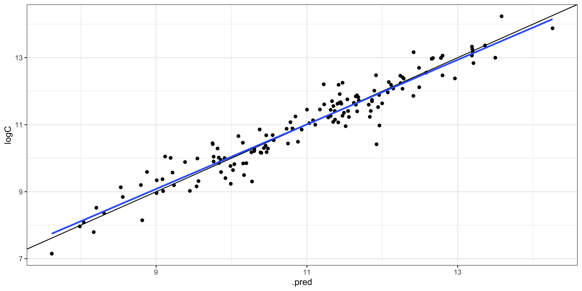

The whole game

Assignment

Starting with the “Whole Game Image” on the last slide, in plain language, write a sentence or 2 about each step and item, its importance, and note key things to be careful of. The full submission should be a 2-3 paragraph narative of the entire process, including the final model fit and performance.

Lecture 19

Recaping Day 1 - 4

Evaluation

Classification:

Confusion matrix

What to do with a confusion matrix

1. Accuracy

2. Sensitivity

3. Specificity

Two class data

Varying the threshold

ROC curves

ROC curves

ROC curves

Brier score

Brier score

Separation vs calibration

Regression

R-squared (\(R^2\))

Root Mean Squared Error (RMSE)

Mean Absolute Error (MAE)

Comparing Metrics

Choosing the Right Metric

Metrics Selection model performance

Recap

Previously - Setup

Previously - Data Usage

Previously - Feature engineering

Optimizing Models via Tuning Hyperparameter

Tuning parameters

Tagging parameters for tuning

Boosted Trees

Boosted Tree Tuning Parameters

Boosted Tree Tuning Parameters

Optimize tuning parameters

1. Grid search

1. Grid search

2. Iterative Search

Grid Search Example

Parameters

Grids

Different types of grids

Create a grid

Create a grid

Create a SFD curve

Create a regular grid

Update parameter ranges

The results

Use the tune_*() functions to tune models

Choosing tuning parameters

Grid Search

Grid Search

Grid results

Tuning results

Choose a parameter combination

Choose a parameter combination

Checking Calibration

The final fit!

The final fit!

The whole game

Assignment

Use the `tune_*()` functions to tune models