library(forecast)

co2_arima <- auto.arima(co2)

summary(co2_arima)
#> Series: co2
#> ARIMA(1,1,1)(1,1,2)[12]
#>
#> Coefficients:
#>          ar1      ma1     sar1     sma1     sma2
#>       0.2569  -0.5847  -0.5489  -0.2620  -0.5123
#> s.e.  0.1406   0.1204   0.5880   0.5701   0.4819
#>
#> sigma^2 = 0.08576:  log likelihood = -84.39
#> AIC=180.78   AICc=180.97   BIC=205.5
#>
#> Training set error measures:
#>                      ME     RMSE       MAE         MPE       MAPE      MASE
#> Training set 0.01742092 0.287159 0.2303994 0.005073769 0.06845665 0.1819636
#>                      ACF1
#> Training set -0.002858162Lecture 22
Introduction to Time Series Forecasting
Monday
- We covered the following topics:
sate-time data in R (date, POSIXct, POSIXlt)
Time series data/structure (ts, tsibble, tibble + Date column)
Time series decomposition
- Trend, seasonality, and residuals
Smoothing time series data
- Smoothing with moving averages
Today
- Forecasting with two distinct models (1) ARIMA (2) Prophet
- Understanding modeltime + tidymodels integration
- Forecasting Process for time series
Toy Example: River Time Series & ARIMA
Let’s say we’re watching how much water flows in a river every day:
- Monday: 50 cfs
- Tuesday: 60 cfs
- Wednesday: 70 cfs
We want to guess tomorrow’s flow.
1. AutoRegressive (AR)
This means: “Look at yesterday and the day before!”
If flow has been going up each day, AR says: ** “Tomorrow might go up again …” **
It’s like the river has a pattern.
2. Integrated (I)
Sometimes the flow just keeps climbing — like during a spring snowmelt!
To help ARIMA think better, we subtract yesterday’s number from today’s.
This makes the numbers more steady so ARIMA can do its magic.
3. Moving Average (MA)
The river sometimes gets a surprise flux (like a big rainstorm 🌧️).
MA looks at those surprises and helps smooth them out.
So if it rained two days ago, MA might say: “Don’t expect another surprise tomorrow.”
Put It All Together: AR + I + MA = ARIMA
- AR: Uses the river’s memory (trend)
- I: Calms the sturcutral components (season)
- MA: Handles noisy surprises (noise)
Now we can forecast tomorrow’s flow!
ARIMA
The basics of a ARIMA (AutoRegressive Integrated Moving Average) Model include:
- AR: AutoRegressive part (past values):
- AR(1) = current value depends on the previous value
- AR(2) = current value depends on the previous two values
- AR(1) = current value depends on the previous value
- I: Integrated part (differencing to make data stationary)
- Differencing removes trends and seasonality
- e.g.,
diff(co2, lag = 12)removes annual seasonality
- Differencing removes trends and seasonality
- MA: Moving Average part (past errors)
- MA(1) = current value depends on the previous error
- MA(2) = current value depends on the previous two errors
- MA(1) = current value depends on the previous error
- p, d, q: Parameters for AR, I, and MA
- p = number of lagged values (AR)
- d = number of differences (I)
- q = number of lagged errors (MA)
- p = number of lagged values (AR)
AIC
The AIC metric helps choose between models/parameters:
- It rewards:
- Good predictions
- Simplicity
- It punishes:
- Complexity (too many parameters)
- Overfitting (fitting noise instead of the trend)
- Lower AIC = better model
A Simple Forecasting Example
auto.arima()is a function from theforecastpackage that automatically selects the best ARIMA model for your data accoridning toe to the AICc criterion.- The AICc (Akaike Information Criterion corrected) is a measure of the relative quality of statistical models for a given dataset.
- It is used to compare different models and select the one that best fits the data while penalizing for complexity.
- The
auto.arima()function will automatically select the best parameters (p,d,q) based on the AICc criterion.
Forecasting with ARIMA
- The
forecast()function is used to generate forecasts from the fitted ARIMA model. - The
hargument specifies the number of periods to forecast into the future.
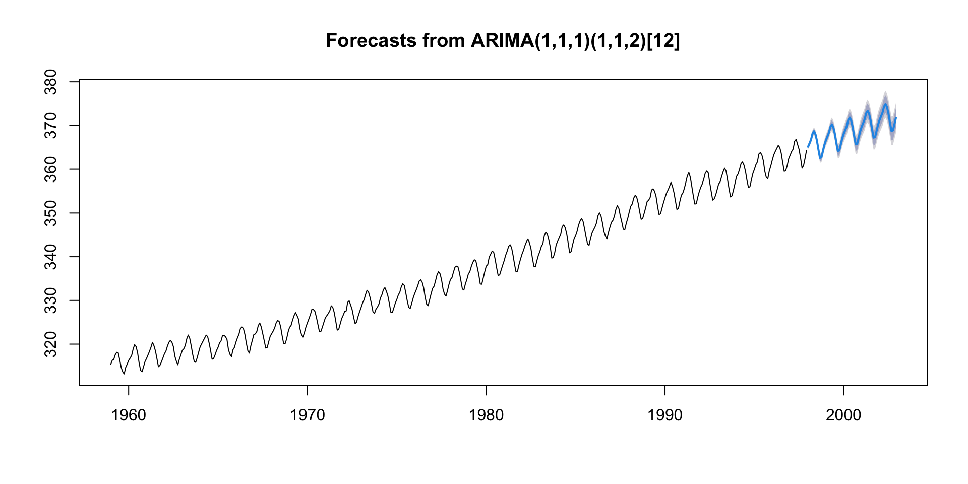
🔢 ARIMA(1,1,1)(1,1,2)[12]
ARIMA Notation can be broken into two parts:
1. Non-seasonal part: ARIMA(1, 1, 1)
This is the “regular” ARIMA: - AR(1): One autoregressive term — the model looks at one lag of the time series.
I(1): One differencing — the model uses the change in values instead of raw values to make the series more stationary.
MA(1): One moving average term — the model corrects using one lag of the error term.
2. Seasonal part: (1, 1, 2)[12]
This is the seasonal pattern — repeated every 12 time units (like months in a year):
SAR(1): One seasonal autoregressive term — it uses the value from 12 time steps ago.
SI(1): One seasonal difference — subtracts the value from 12 steps ago to remove seasonal patterns.
SMA(2): Two seasonal moving average terms — uses errors from 12 and 24 time steps ago.
[12]: This is the seasonal period, i.e., it’s a yearly pattern with monthly data.
🔢 ARIMA(1,1,1)(1,1,2)[12]
Hey, ARIMA please…
“Model the data using a mix of its last value, the last error, and their seasonal versions from 12 months ago — but first difference it once to remove trend and once seasonally to remove yearly patterns.”
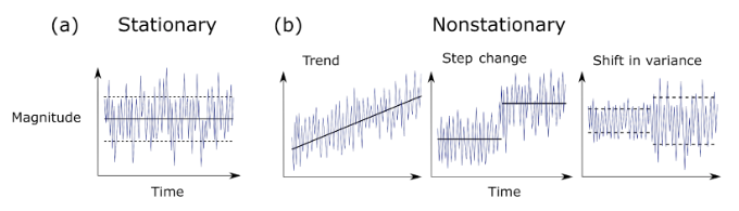
Note
ARIMA modeling works well when data is stationary. - Stationarity means the statistical properties of the series (mean, variance) do not change over time. - Non-stationary data can lead to unreliable forecasts and misleading results.
Prophet
Prophet is an open-source tool for forecasting time series data.
Developed by Facebook (Meta)
Designed for analysts and data scientists
Handles missing data, outliers, and seasonality
Key Features of Prophet
✅ Additive Model: Trend + Seasonality + Holidays + Noise
✅ Automatic Changepoint Detection
✅ Support for Custom Holidays & Events
✅ Flexible Seasonality (daily/weekly/yearly)
✅ Easy-to-use API in R and Python
Prophet’s Model Structure
Prophet decomposes time series into components:
\[ y(t) = g(t) + s(t) + h(t) + ε(t) \]
g(t): Trend (linear or logistic growth)
s(t): Seasonality (Fourier series)
h(t): Holiday effects
ε(t): Error term (noise)
📌 Assumes additive components by default; multiplicative also possible
A Simple Forecasting Example
Your time series must have: (1) ds column (date/timestamp) (2) y column (value to forecast)
Pros / Cons
| Feature | ARIMA | Prophet |
|---|---|---|
| Statistical rigor | Based on strong statistical theory; well-studied | Intuitive, decomposable model (trend + seasonality + events) |
| Interpretability | Clear interpretation of AR, MA, differencing terms | Plots components like trend/seasonality directly |
| Flexibility (SARIMA) | Seasonal ARIMA can handle seasonal structure | Handles multiple seasonalities natively (yearly, weekly, daily) |
| Control over params | Fine-tuned control over differencing, lags, and model order | Easy to specify changepoints, seasonality, and custom events |
| Statistical testing | Includes AIC/BIC for model selection | Cross-validation support; uncertainty intervals included |
| Requires stationarity | Time series must be stationary or made so (differencing) | Handles non-stationary data out of the box |
| Model complexity | Needs careful tuning (p,d,q) and domain expertise | Defaults work well; limited tuning needed |
| Holiday effects | Must be encoded manually | Easy to include holidays/events |
| Multivariate support | Basic ARIMA doesn’t support exogenous variables easily (need ARIMAX) | Supports external regressors with add_regressor() |
| Non-linear trends | Poor performance with structural breaks or non-linear growth | Handles changepoints and logistic growth models well |
| Seasonality limits | SARIMA handles only one seasonal period well | Built-in multiple seasonal components (e.g., daily, weekly, yearly) |
TL;DR
- Use ARIMA if you want a classic, statistical model with deep customization and you’re comfortable making your data stationary.
- Use Prophet if you want a fast, robust, and intuitive model for business or environmental data with strong seasonal effects and irregular events.
To much complexity!!
Each model has it own requirements, arguments, and tuning parameters.
Simular to our ML models, this introduces a large time sink, opportunity for error, and complexity.
modeltimebrings tidy workflows to time series forecasting using theparsnipandworkflowsframeworks fromtidymodels.Combine multiple models (ARIMA, Prophet, XGBoost) in one framework to
Modeltime Integration ![]()
![]()


1. Create a time series split …
Use
time_series_split()to make a train/test set.Setting assess = “…” tells the function to use the last … of data as the testing set.
Setting cumulative =
TRUEtells the sampling to use all of the prior data as the training set.
2. Specify Models …
Just like tidymodels …
Model Spec:
arima_reg()/prophet_reg()/prophet_boost()<– This sets up your general model algorithm and key parametersModel Mode:
mode = "regression"/mode = "classification"<– This sets the model mode to regression or classification (timeseries is always regression!)Set Engine:
set_engine("auto_arima")/set_engine("prophet")/ <– This selects the specific package-function to use, you can add any function-level arguments here.
mods <- list(
  arima_reg() |>  set_engine("auto_arima"),

  arima_boost(min_n = 2, learn_rate = 0.015) |> set_engine(engine = "auto_arima_xgboost"),

  prophet_reg() |> set_engine("prophet"),

  prophet_boost() |> set_engine("prophet_xgboost"),

  # Exponential Smoothing State Space model
  exp_smoothing() |> set_engine(engine = "ets"),

  # Multivariate Adaptive Regression Spline model
  mars(mode = "regression") |> set_engine("earth")
)
3. Fit Models …
Use
purrr::map()tofitthemodelsto the training data.Fit Model: fit(value ~ date, training) <– All
modeltimemodels require a date column to be a regressor.
4. Build modeltime table …
- Use
modeltime_table()to combine multiple models into a single table that can be used for calibration, accuracy, and forecasting.
modeltime_table():
Creates a table of models
Validates that all objects are models (parsnip or workflows objects) and all models have been fitted
Provides an ID and Description of the models
as_modeltime_table():
- Converts a list of models to a modeltime table. Useful if programatically creating Modeltime Tables from models stored in a list (e.g. from
map).
(models_tbl <- as_modeltime_table(models))
#> # Modeltime Table
#> # A tibble: 6 × 3
#>   .model_id .model   .model_desc
#>       <int> <list>   <chr>
#> 1         1 <fit[+]> ARIMA(1,1,1)(2,1,2)[12]
#> 2         2 <fit[+]> ARIMA(1,1,1)(0,1,1)[12]
#> 3         3 <fit[+]> PROPHET
#> 4         4 <fit[+]> PROPHET
#> 5         5 <fit[+]> ETS(M,A,A)
#> 6         6 <fit[+]> EARTH
Notes:
modeltime_table() does some basic checking to ensure all models are fit and organized into a scalable structure called a “Modeltime Table” that is used as part of our forecasting workflow.
- It’s expected that tuning and parameter selection is performed prior to incorporating into a Modeltime Table.
- If you try to add an unfitted model, the
modeltime_table()will complain (throw an informative error) saying you need to fit() the model.
5. Calibrate the Models …
Use
modeltime_calibrate()to evaluate the models on the test set.Calibrating adds a new column,
.calibration_data, with the test predictions and residuals inside.
(calibration_table <- modeltime_calibrate(models_tbl, testing, quiet = FALSE))
#> # Modeltime Table
#> # A tibble: 6 × 5
#>   .model_id .model   .model_desc             .type .calibration_data
#>       <int> <list>   <chr>                   <chr> <list>
#> 1         1 <fit[+]> ARIMA(1,1,1)(2,1,2)[12] Test  <tibble [60 × 4]>
#> 2         2 <fit[+]> ARIMA(1,1,1)(0,1,1)[12] Test  <tibble [60 × 4]>
#> 3         3 <fit[+]> PROPHET                 Test  <tibble [60 × 4]>
#> 4         4 <fit[+]> PROPHET                 Test  <tibble [60 × 4]>
#> 5         5 <fit[+]> ETS(M,A,A)              Test  <tibble [60 × 4]>
#> 6         6 <fit[+]> EARTH                   Test  <tibble [60 × 4]>
A few notes on Calibration:
Calibration builds confidence intervals and accuracy metrics
Calibration Data is the predictions and residuals that are calculated from out-of-sample data.
After calibrating, the calibration data follows the data through the forecasting workflow.
Testing Forecast & Accuracy Evaluation
There are 2 critical parts to an evaluation.
- Evaluating the Test (Out of Sample) Accuracy
- Visualizing the Forecast vs Test Data Set
Accuracy
modeltime_accuracy() collects common accuracy metrics using yardstick functions:
- MAE - Mean absolute error, mae()
- MAPE - Mean absolute percentage error, mape()
- MASE - Mean absolute scaled error, mase()
- SMAPE - Symmetric mean absolute percentage error, smape()
- RMSE - Root mean squared error, rmse()
- RSQ - R-squared, rsq()
modeltime_accuracy(calibration_table) |>
arrange(mae)
#> # A tibble: 6 × 9
#> .model_id .model_desc .type mae mape mase smape rmse rsq
#> <int> <chr> <chr> <dbl> <dbl> <dbl> <dbl> <dbl> <dbl>
#> 1 1 ARIMA(1,1,1)(2,1,2)[12] Test 0.810 0.224 0.687 0.224 0.967 0.973
#> 2 2 ARIMA(1,1,1)(0,1,1)[12] Test 0.885 0.244 0.750 0.245 1.05 0.969
#> 3 3 PROPHET Test 1.06 0.295 0.899 0.294 1.16 0.986
#> 4 4 PROPHET Test 1.06 0.295 0.899 0.294 1.16 0.986
#> 5 5 ETS(M,A,A) Test 1.48 0.409 1.25 0.410 1.71 0.958
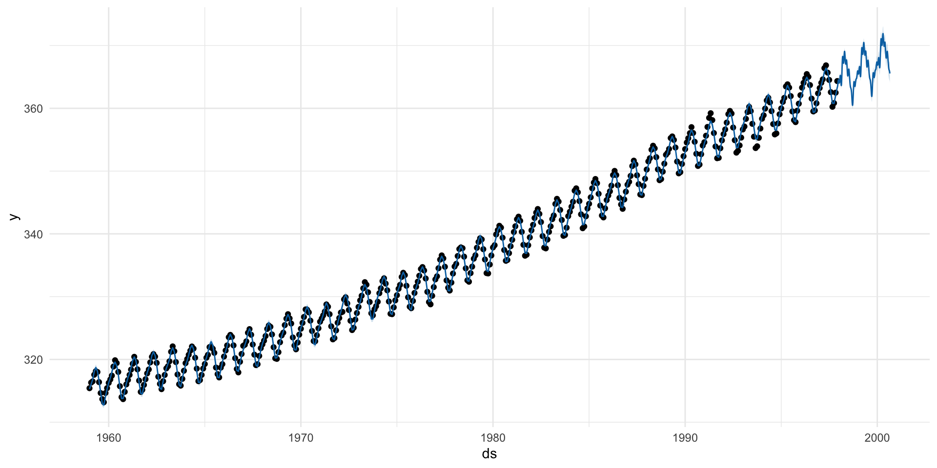
#> 6 6 EARTH Test 1.89 0.526 1.61 0.526 2.25 0.499Forecast
- Use
modeltime_forecast()to generate forecasts for the next 120 months (10 years). - Use
plot_modeltime_forecast()to visualize the forecasts.
(forecast <- calibration_table  |>
  modeltime_forecast(h = "60 months",
                     new_data = testing,
                     actual_data = co2_tbl) )
#> # Forecast Results
#>
#> # A tibble: 828 × 7
#>    .model_id .model_desc .key   .index     .value .conf_lo .conf_hi
#>        <int> <chr>       <fct>  <date>      <dbl>    <dbl>    <dbl>
#>  1        NA ACTUAL      actual 1959-01-01   315.       NA       NA
#>  2        NA ACTUAL      actual 1959-02-01   316.       NA       NA
#>  3        NA ACTUAL      actual 1959-03-01   316.       NA       NA
#>  4        NA ACTUAL      actual 1959-04-01   318.       NA       NA
#>  5        NA ACTUAL      actual 1959-05-01   318.       NA       NA
#>  6        NA ACTUAL      actual 1959-06-01   318        NA       NA
#>  7        NA ACTUAL      actual 1959-07-01   316.       NA       NA
#>  8        NA ACTUAL      actual 1959-08-01   315.       NA       NA
#>  9        NA ACTUAL      actual 1959-09-01   314.       NA       NA
#> 10        NA ACTUAL      actual 1959-10-01   313.       NA       NA
#> # ℹ 818 more rows
Vizualize
Refit to Full Dataset & Forecast Forward
The final step is to refit the models to the full dataset using modeltime_refit() and forecast them forward.
Why refit?
The models have all changed! This is the (potential) benefit of refitting.
More often than not refitting is a good idea. Refitting:
Retrieves your model and preprocessing steps
Refits the model to the new data
Recalculates any automations. This includes:
- Recalculating the changepoints for the Earth Model
- Recalculating the ARIMA and ETS parameters
Preserves any parameter selections. This includes:
Any other defaults that are not automatic calculations are used.
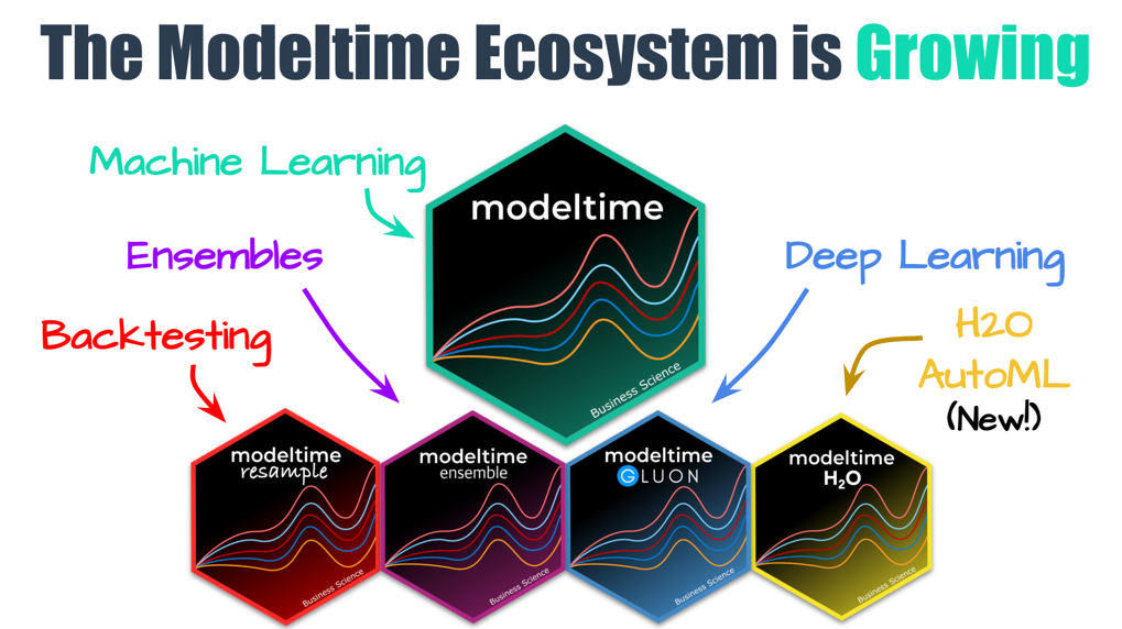
Growing Ecosystem
Summary & Takeaways
Environmental science is rich with time series applications
Time series data is sequential and ordered
lubridatesimplifies handling and extracting date-time featuresUse
ts,zoo,xtsfor classic or irregular dataUse
tsibble,feasts, andfablefor tidy workflowsLearn to decompose, smooth, and forecast
Use
modeltimefor advanced modeling and forecasting
Assignment
- Use
modeltimeto forecast the next 12 months of streamflow data in the Poudre River based on last time assignment. - Use the
prophet_reg(), andarima_reg()function to create a Prophet model for forecasting. - Use dataRetrieval to download daily streamflow for the next 12 months. Aggregate this data to monthly averages and compare it to the predictions made by your modeltime model.
- Compute the R2 value between the model predictions and the observed data using a linear model and report the meaning.
- Last, generate a plot of the Predicted vs Observed values and include a 1:1 line, and a linear model line.