Lecture 23
Introduction to Simple Features
Spatial Data
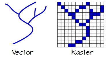
To work in a GIS environment, real world features (objects or phenomena that can be recorded in 2D or 3D space) need to be reduced to spatial entities.
These spatial entities can be represented using as a vector data model (this week) or a raster data model (next week).
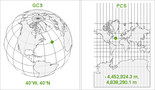
Projections
- Projections can have angular units (lat/lon) - geographic coordinate systems (GCS)
or
- Projections can have distance units (m) - projected coordinate systems (PCS)
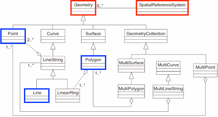
Simple Features Model
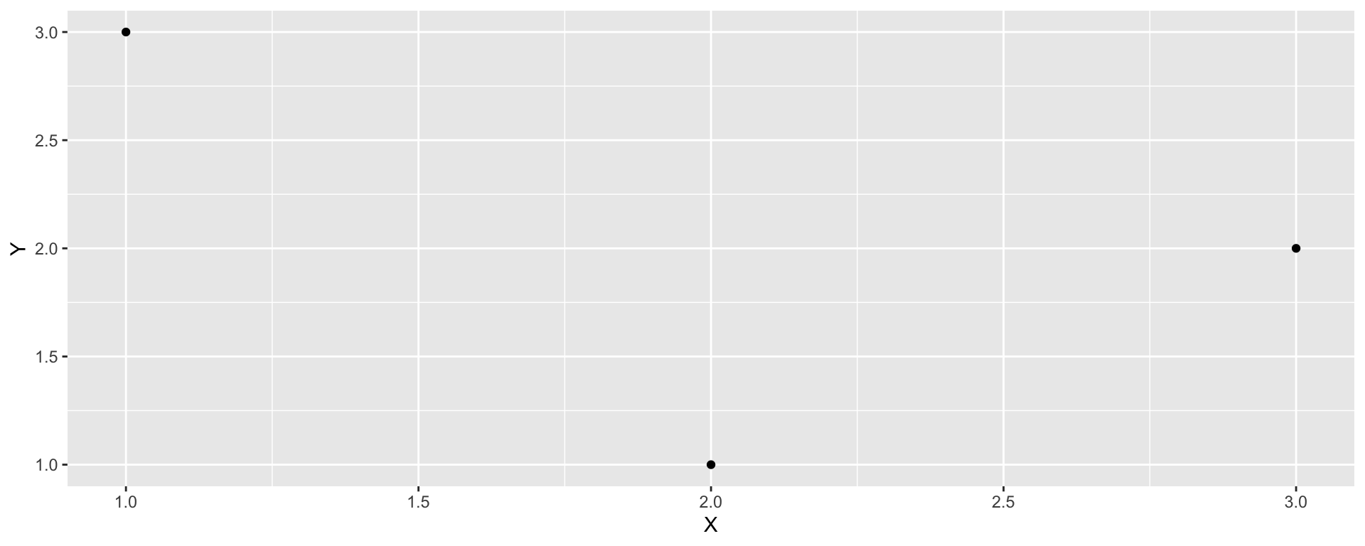
Points
A point is composed of one coordinate pair in a specific coordinate system.
Points have no length or area.
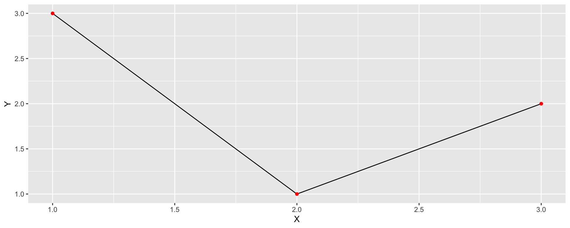
LINESTRING
A linestring is composed of a ordered sequence of two or more coordinate points
Points in a line are called vertices and explicitly define the connection between two points.
A line has length, but no area
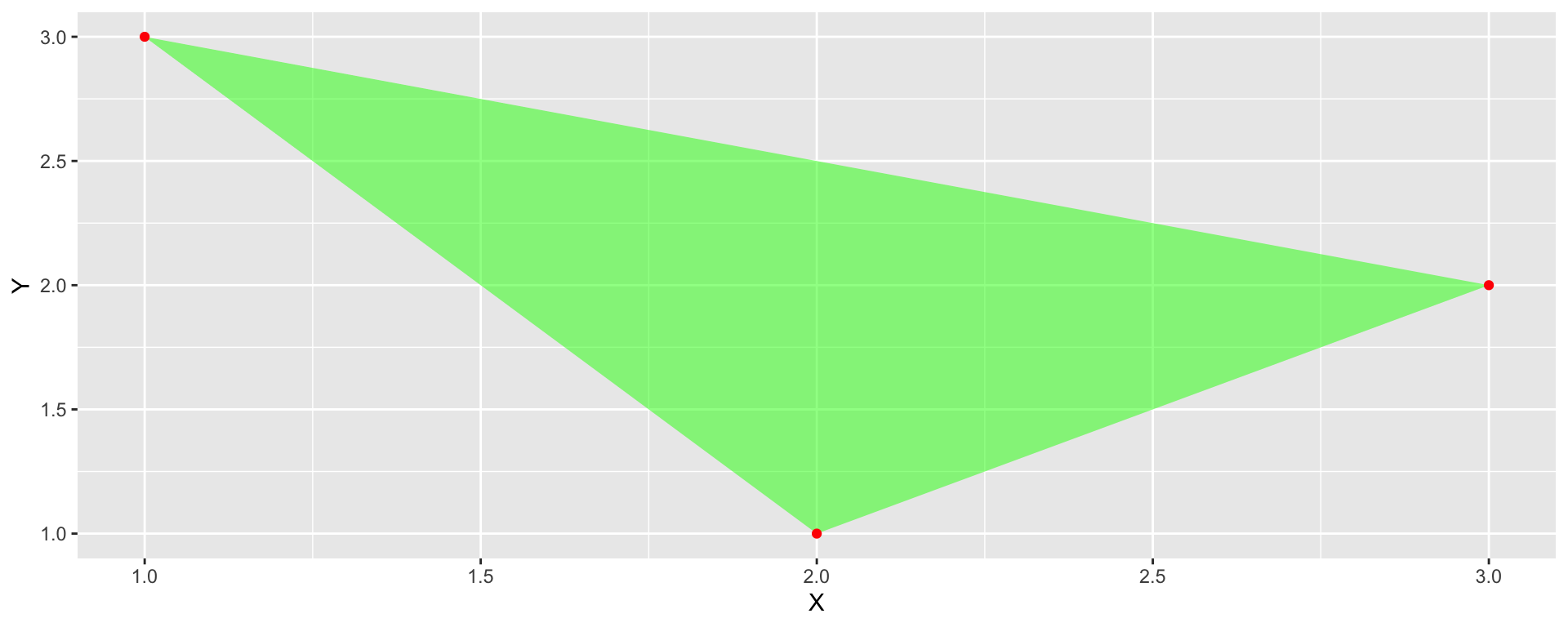
POLYGON
A polygon is composed of 4 or more points whose starting and ending point are the same.
Polygons have both length and area.
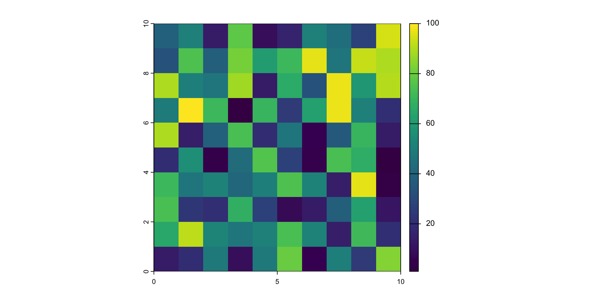
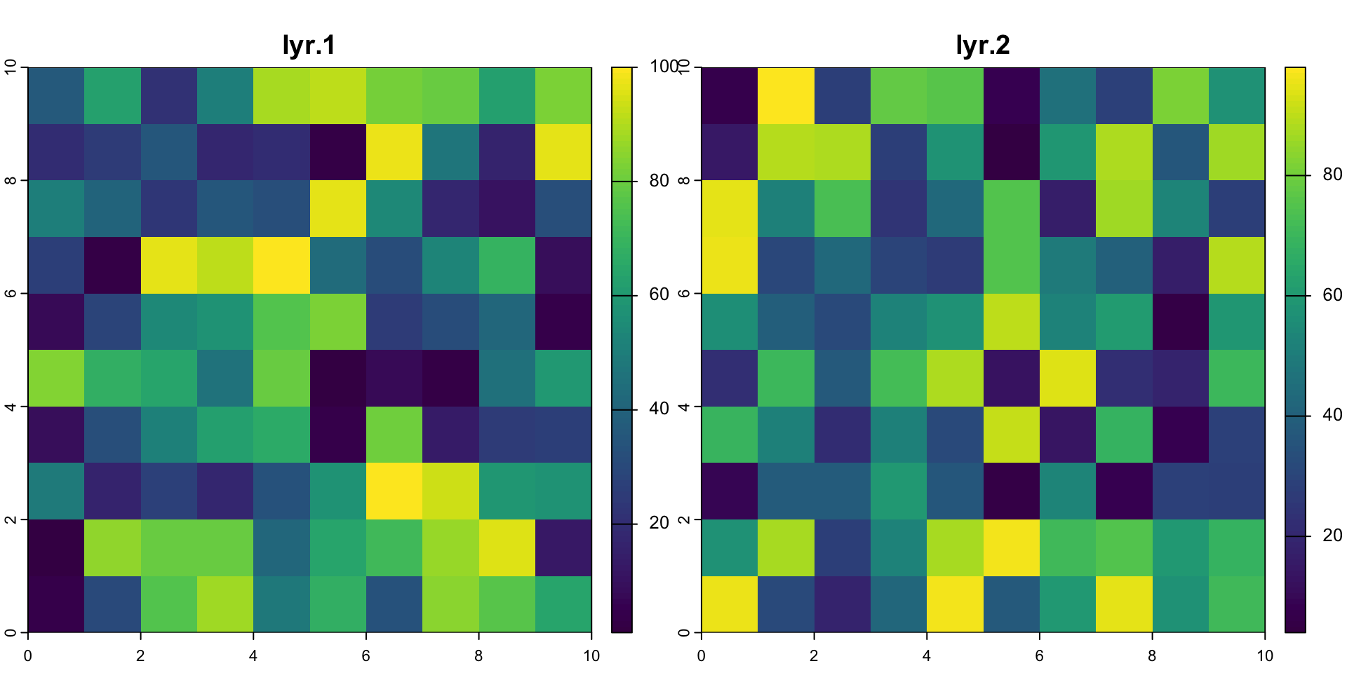
Raster
The raster data model uses an array of cells to represent real-world phenomena and is defined by a resolution (X and Y dimension of the cells), extent and and CRS.
Raster datasets are commonly used for representing and managing imagery, climate data, elevation models, and other entities.
Today: Simple features
Simple Features (officially Simple Feature Access) is both an OGC and International Organization for Standardization (ISO) standard that specifies a common storage and access model of (mostly) two-dimensional geometries.
Simple features (sf) package
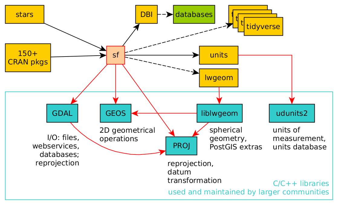
Simple Features
sf, sfc, sfg
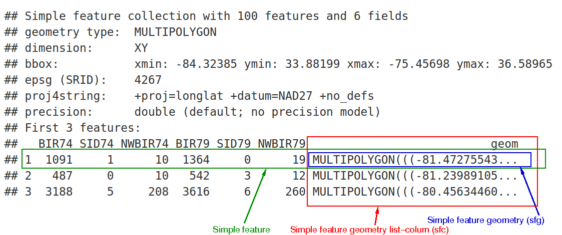
In the output we see:
in green a simple feature: a single record (row, consisting of attributes and geometry
in blue a single simple feature geometry (an object of class
sfg)in red a simple feature list-column (an object of class
sfc, which is a column in thedata.frame)Even though geometries are native R objects, they are printed as well-known text
Conversion between types
Lets take the Larimer County in our Colorado sf object:
(co1 = AOI::aoi_get(state = "CO", county = "Larimer")$geometry)
#> Geometry set for 1 feature
#> Geometry type: MULTIPOLYGON
#> Dimension:     XY
#> Bounding box:  xmin: -106.1954 ymin: 40.25778 xmax: -104.9431 ymax: 40.99844
#> Geodetic CRS:  WGS 84
#> MULTIPOLYGON (((-105.6533 40.26046, -105.6094 4...
(co_ls = st_cast(co1, "MULTILINESTRING"))
#> Geometry set for 1 feature
#> Geometry type: MULTILINESTRING
#> Dimension:     XY
#> Bounding box:  xmin: -106.1954 ymin: 40.25778 xmax: -104.9431 ymax: 40.99844
#> Geodetic CRS:  WGS 84
#> MULTILINESTRING ((-105.6533 40.26046, -105.6094...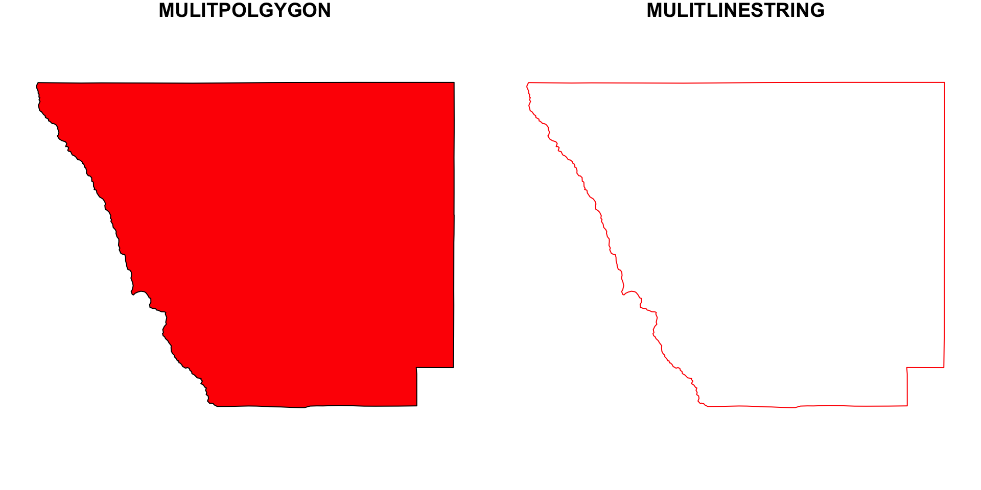
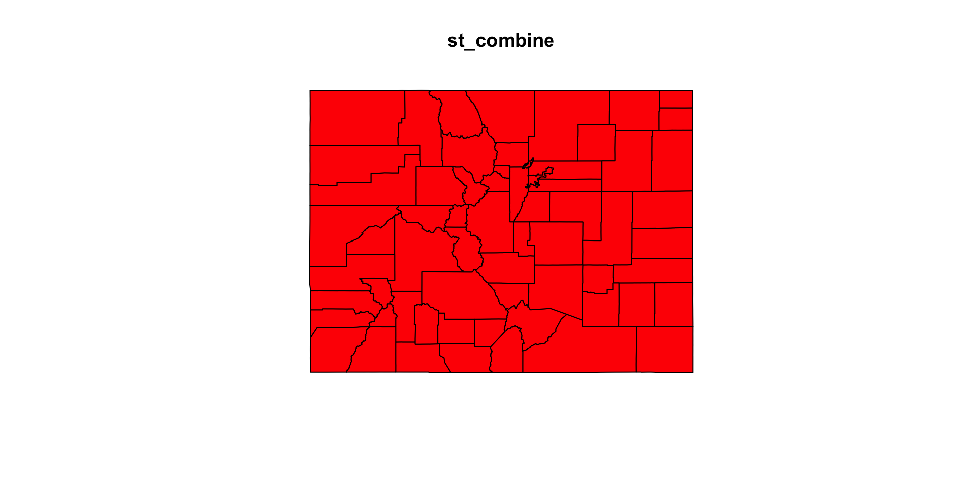
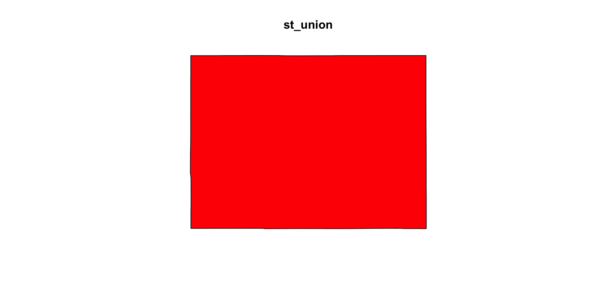
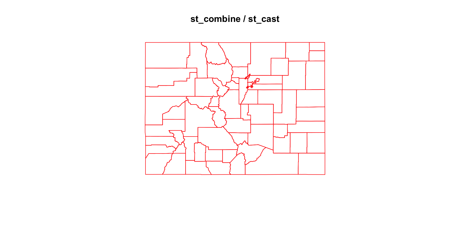
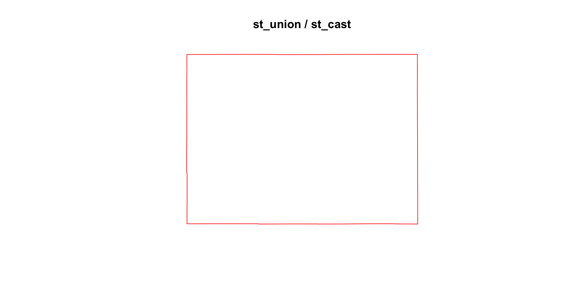
Disolving Geometries Boundaries
Combining geometries preserves their interior boundaries, unioning dissolves the internal boundaries:
(co_geom = co$geometry)
#> Geometry set for 64 features
#> Geometry type: MULTIPOLYGON
#> Dimension:     XY
#> Bounding box:  xmin: -109.0602 ymin: 36.99246 xmax: -102.0415 ymax: 41.00342
#> Geodetic CRS:  WGS 84
#> First 5 geometries:
#> MULTIPOLYGON (((-105.0532 39.79106, -104.976 39...
#> MULTIPOLYGON (((-105.4855 37.5779, -105.4859 37...
#> MULTIPOLYGON (((-103.7065 39.73989, -103.7239 3...
#> MULTIPOLYGON (((-107.1287 37.42294, -107.2803 3...
#> MULTIPOLYGON (((-102.0416 37.64428, -102.0558 3...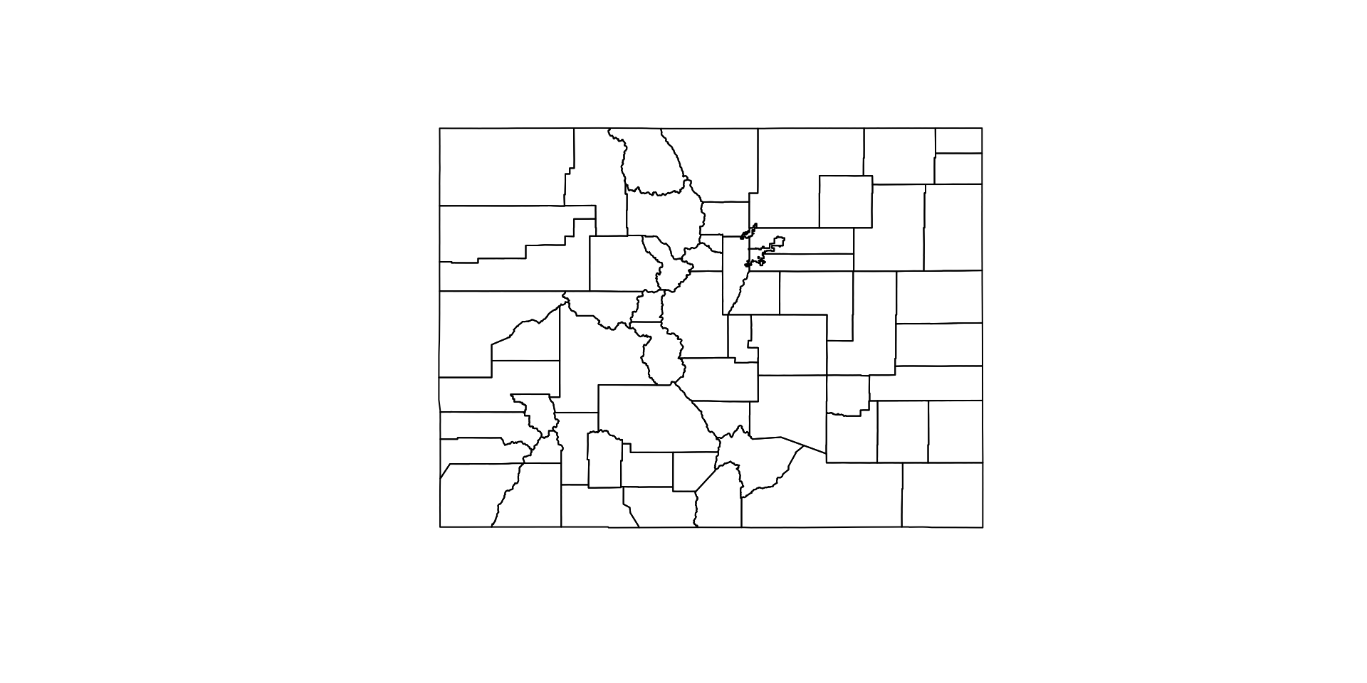
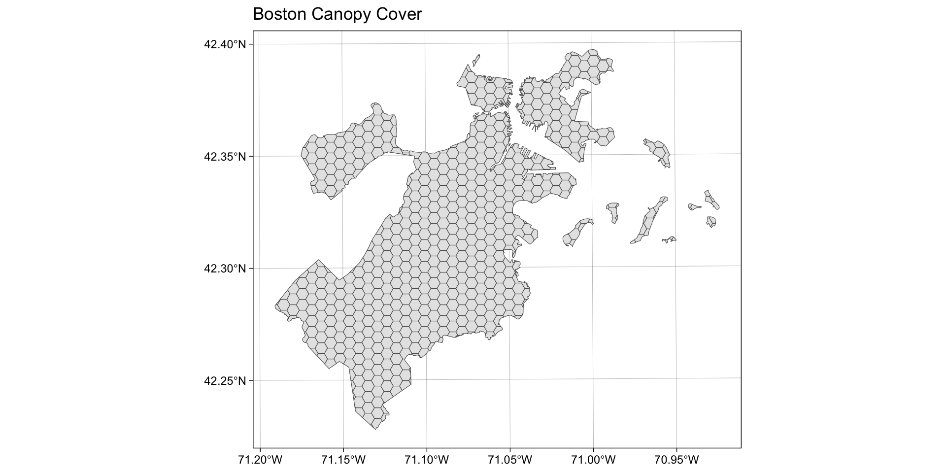
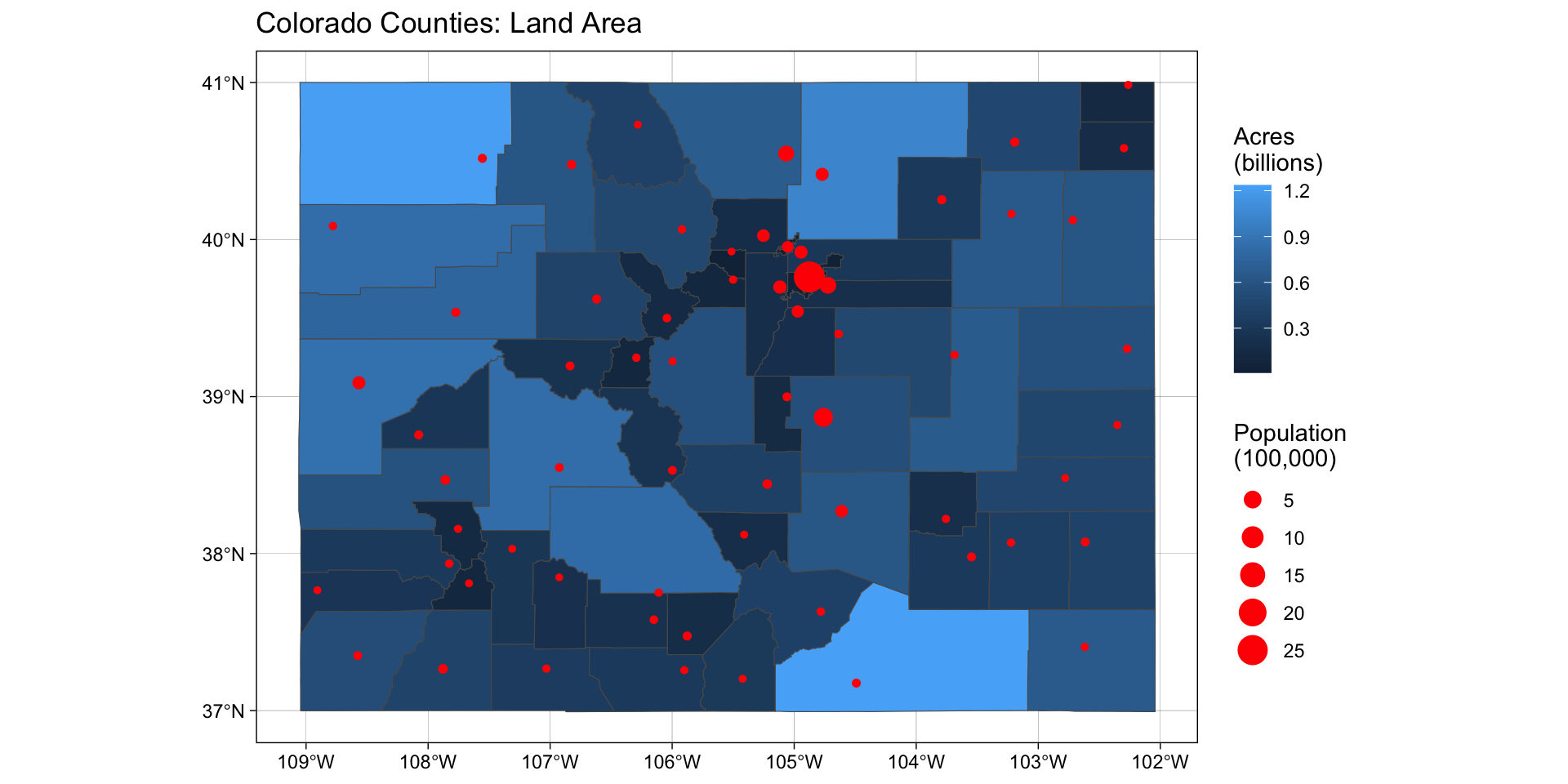
sf an ggplot

sf an ggplot
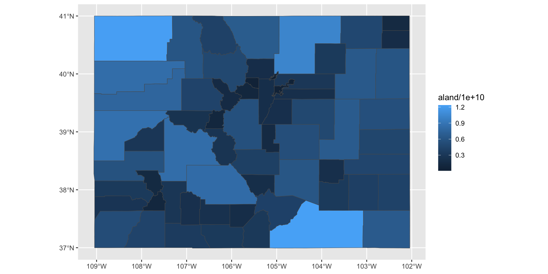
sf an ggplot
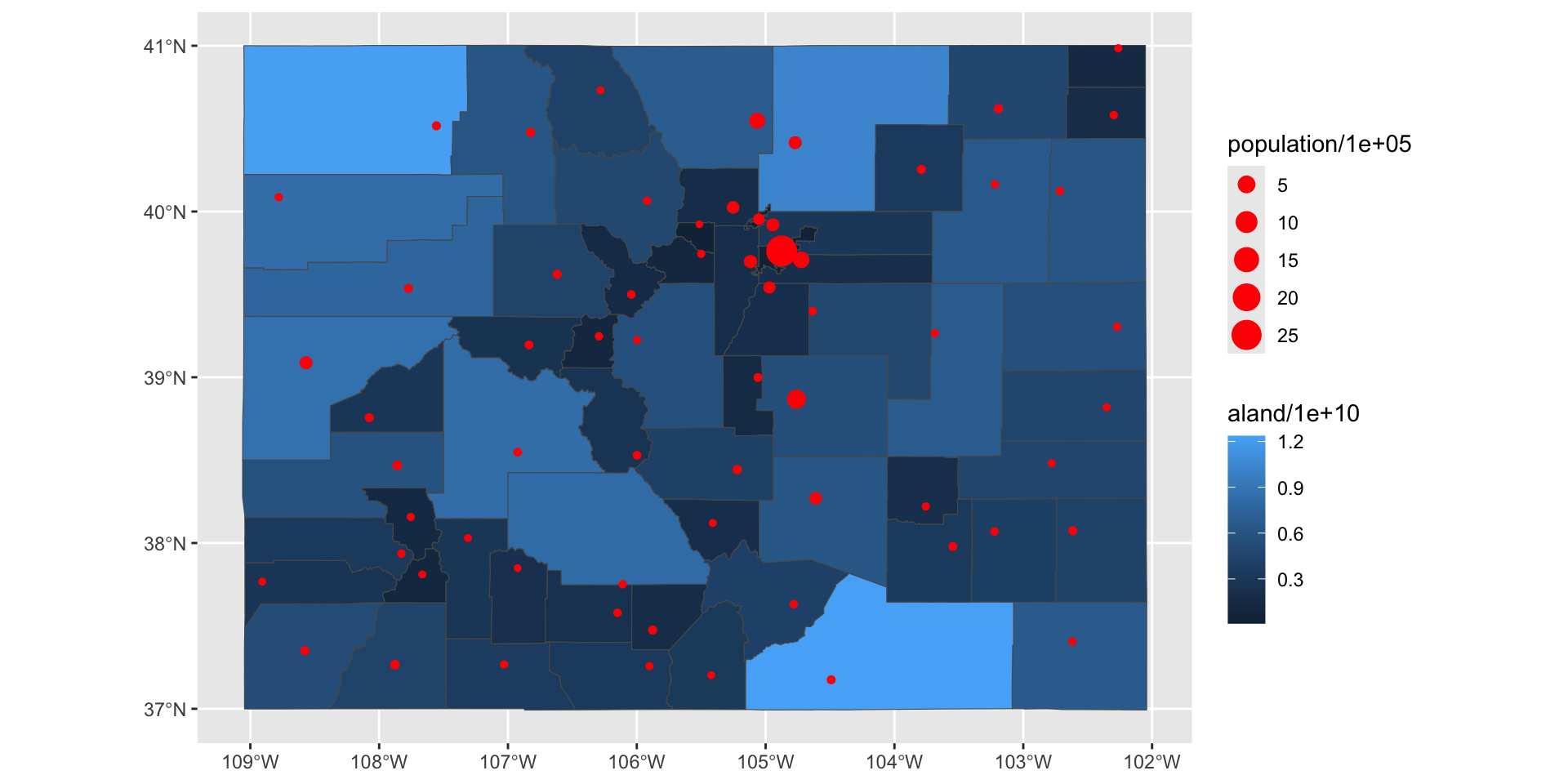
sf an ggplot
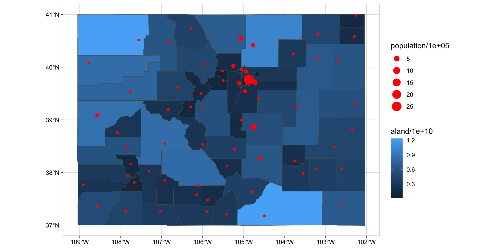
sf an ggplot
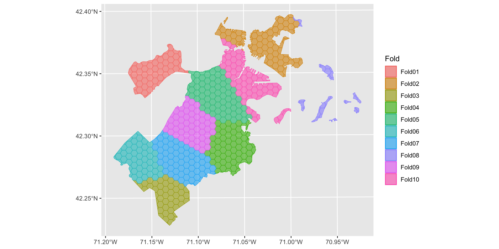
Spatial Sampling
- Spatial sampling is a common task in spatial data science.
Like
rsample,spatialsampleprovides building blocks for creating and analyzing resamples of a spatial data set but does not include code for modeling or computing statistics.