As we’ve seen above, reading spatial data from an external file can be done via sf
co <-read_sf("data/co.shp")
Writing takes place in the same fashion, using write_sf:
write_sf(co, "co.shp") # silently overwrites
From Tables (e.g. CSV)
Spatial data can also be created from CSV and other flat files once it is in R:
(cities =read_csv("../labs/data/uscities.csv") |>select(city, state_name, county_name, population, lat, lng) )#> # A tibble: 31,254 × 6#> city state_name county_name population lat lng#> <chr> <chr> <chr> <dbl> <dbl> <dbl>#> 1 New York New York Queens 18832416 40.7 -73.9#> 2 Los Angeles California Los Angeles 11885717 34.1 -118. #> 3 Chicago Illinois Cook 8489066 41.8 -87.7#> 4 Miami Florida Miami-Dade 6113982 25.8 -80.2#> 5 Houston Texas Harris 6046392 29.8 -95.4#> 6 Dallas Texas Dallas 5843632 32.8 -96.8#> 7 Philadelphia Pennsylvania Philadelphia 5696588 40.0 -75.1#> 8 Atlanta Georgia Fulton 5211164 33.8 -84.4#> 9 Washington District of Columbia District of Columb… 5146120 38.9 -77.0#> 10 Boston Massachusetts Suffolk 4355184 42.3 -71.1#> # ℹ 31,244 more rows
To do this, you must specify the X and the Y coordinate columns as well as a CRS:
A typical lat/long CRS is EPSG:4326
(cities_sf <-st_as_sf(cities, coords =c("lng", "lat"), crs =4326))#> Simple feature collection with 31254 features and 4 fields#> Geometry type: POINT#> Dimension: XY#> Bounding box: xmin: -176.6295 ymin: 17.9559 xmax: 174.111 ymax: 71.2727#> Geodetic CRS: WGS 84#> # A tibble: 31,254 × 5#> city state_name county_name population geometry#> * <chr> <chr> <chr> <dbl> <POINT [°]>#> 1 New York New York Queens 18832416 (-73.9249 40.6943)#> 2 Los Angeles California Los Angeles 11885717 (-118.4068 34.1141)#> 3 Chicago Illinois Cook 8489066 (-87.6866 41.8375)#> 4 Miami Florida Miami-Dade 6113982 (-80.2101 25.784)#> 5 Houston Texas Harris 6046392 (-95.3885 29.786)#> 6 Dallas Texas Dallas 5843632 (-96.7667 32.7935)#> 7 Philadelphia Pennsylvania Philadelph… 5696588 (-75.1339 40.0077)#> 8 Atlanta Georgia Fulton 5211164 (-84.422 33.7628)#> 9 Washington District of Co… District o… 5146120 (-77.0163 38.9047)#> 10 Boston Massachusetts Suffolk 4355184 (-71.0852 42.3188)#> # ℹ 31,244 more rows
Data Manipulation
Since sf objects are data.frames, our dplyr verbs work!
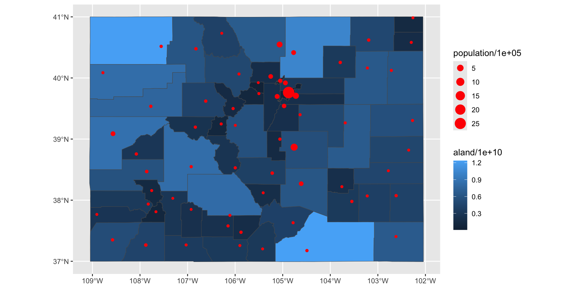
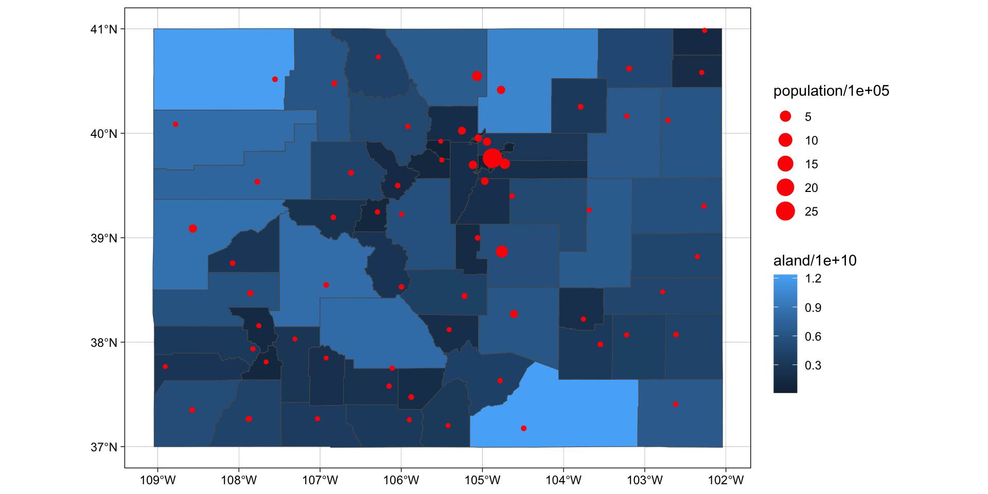
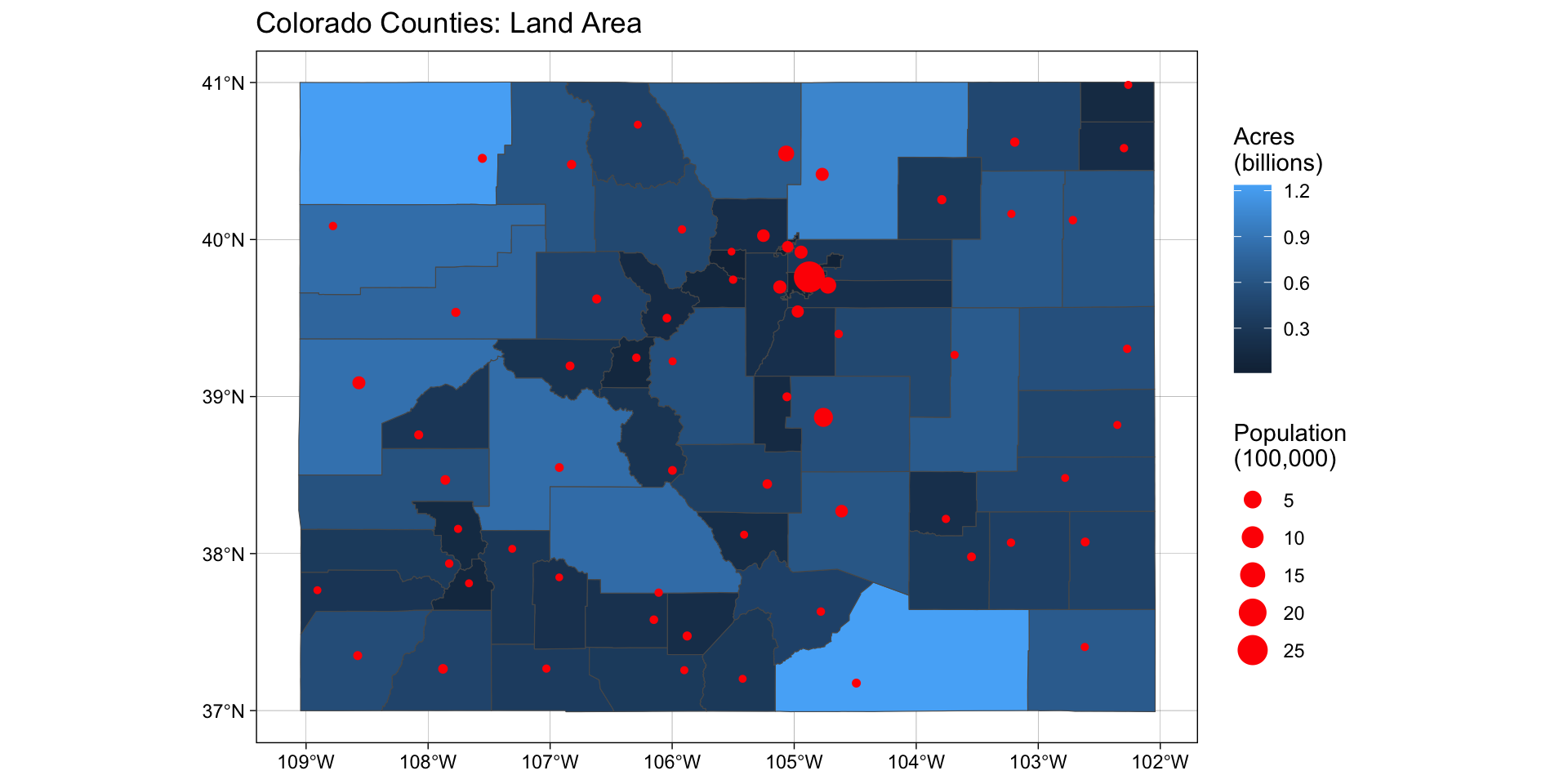
Lets find the most populous city in each Colorado county…
sf and dplyr
cities_sf
#> Simple feature collection with 31254 features and 4 fields
#> Geometry type: POINT
#> Dimension:     XY
#> Bounding box:  xmin: -176.6295 ymin: 17.9559 xmax: 174.111 ymax: 71.2727
#> Geodetic CRS:  WGS 84
#> # A tibble: 31,254 × 5
#>    city         state_name      county_name population            geometry
#>  * <chr>        <chr>           <chr>            <dbl>         <POINT [°]>
#>  1 New York     New York        Queens        18832416  (-73.9249 40.6943)
#>  2 Los Angeles  California      Los Angeles   11885717 (-118.4068 34.1141)
#>  3 Chicago      Illinois        Cook           8489066  (-87.6866 41.8375)
#>  4 Miami        Florida         Miami-Dade     6113982   (-80.2101 25.784)
#>  5 Houston      Texas           Harris         6046392   (-95.3885 29.786)
#>  6 Dallas       Texas           Dallas         5843632  (-96.7667 32.7935)
#>  7 Philadelphia Pennsylvania    Philadelph…    5696588  (-75.1339 40.0077)
#>  8 Atlanta      Georgia         Fulton         5211164   (-84.422 33.7628)
#>  9 Washington   District of Co… District o…    5146120  (-77.0163 38.9047)
#> 10 Boston       Massachusetts   Suffolk        4355184  (-71.0852 42.3188)
#> # ℹ 31,244 more rows
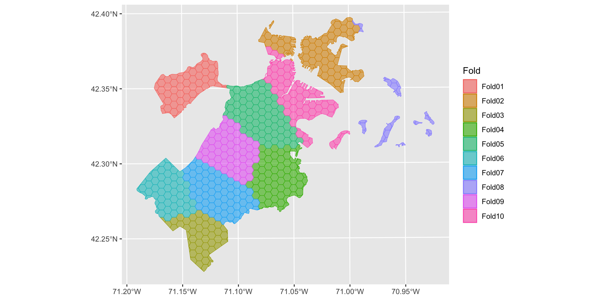
Spatial sampling is a common task in spatial data science.
Like rsample, spatialsample provides building blocks for creating and analyzing resamples of a spatial data set but does not include code for modeling or computing statistics.
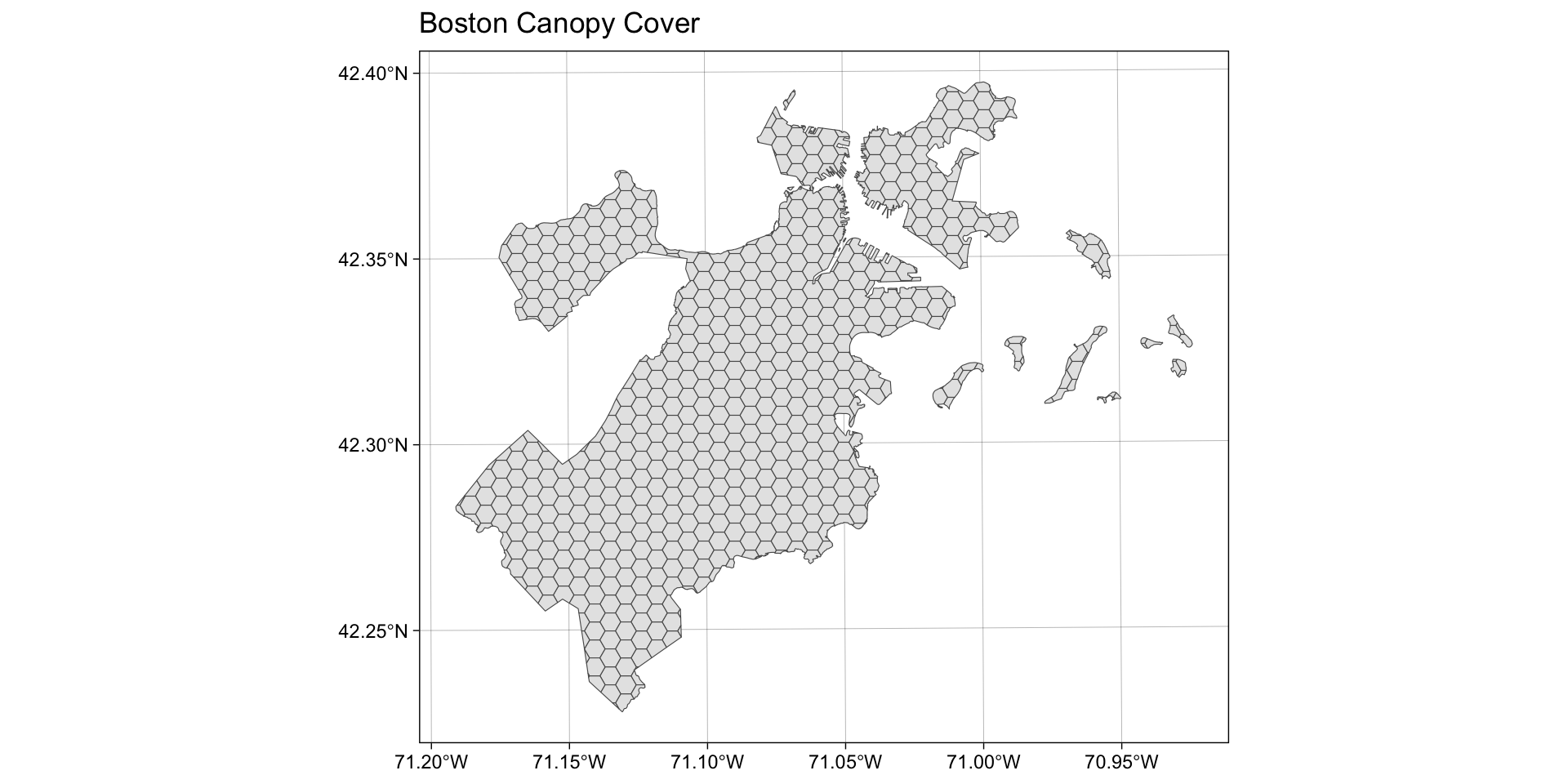
set.seed(1234)folds <-spatial_clustering_cv(boston_canopy, v =10)autoplot(folds)
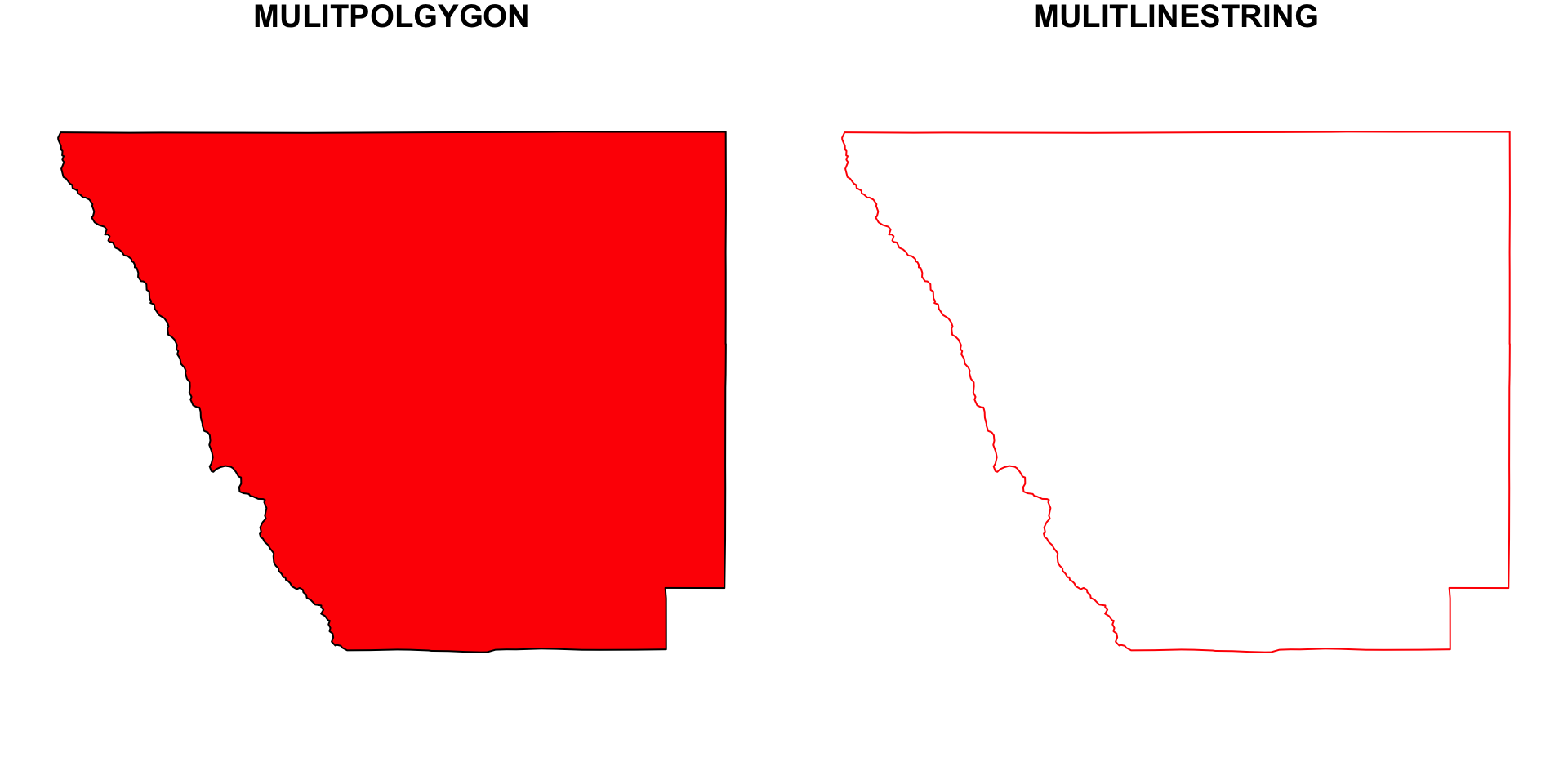
The stickness of sfc column
Geometry columns are “sticky” meaning they persist through data manipulation:
co |>select(name) |>slice(1:2)#> Simple feature collection with 2 features and 1 field#> Geometry type: MULTIPOLYGON#> Dimension: XY#> Bounding box: xmin: -106.0393 ymin: 37.3562 xmax: -103.7057 ymax: 40.00137#> Geodetic CRS: WGS 84#> # A tibble: 2 × 2#> name geometry#> <chr> <MULTIPOLYGON [°]>#> 1 Adams (((-105.0532 39.79106, -105.0532 39.86362, -105.0529 39.91422, -105.0…#> 2 Alamosa (((-105.4855 37.5779, -105.4907 37.57546, -105.4961 37.57006, -105.49…
Dropping the geometry column requires dropping the geometry via sf:
co |>st_drop_geometry() |>#<<select(name) |>slice(1:2)#> # A tibble: 2 × 1#> name #> <chr> #> 1 Adams #> 2 Alamosa
Or cohersing the sf object to a data.frame:
co |>as.data.frame() |>#<<select(name) |>slice(1:2)#> name#> 1 Adams#> 2 Alamosa
Coordinate Systems: What makes spatial data spatial?
What makes a feature geometry spatial is the reference system…
Coordinate Systems
Coordinate Reference Systems (CRS) define how spatial features relate to the surface of the Earth.
CRSs are either geographic or projected…
CRSs are measurement units for coordinates…
sf tools
In sf we have three tools for exploring, define, and changing CRS systems:
st_crs : Retrieve coordinate reference system from sf or sfc object
st_set_crs : Set or replace coordinate reference system from object
st_transform : Transform or convert coordinates of simple feature
Again, “st” (like PostGIS) denotes it is an operation that can work on a ” s patial t ype”
Geographic Coordinate Systms (GCS)
A GCS identifies locations on the curved surface of the earth.
Locations are measured in angular units from the center of the earth relative to the plane defined by the equator and the plane defined by the prime meridian.
The vertical angle describes the latitude and the horizontal angle the longitude
In most coordinate systems, the North-South and East-West directions are encoded as +/-.
North and East are positive (+) and South and West are negative (-) sign.
Geographic Coordinate Systms (GCS)
A GCS is defined by 3 mathematical models of the earth’s shape:
an ellipsoid: earth’s surface that is smooth
defined by two radii: semi-major and semi-minor axes
a geoid: earth’s surface that is undulating
defined by the gravitational potential of the earth
a datum: earth’s surface that is aligned to the geoid
defined by the alignment of the ellipsoid to the geoid
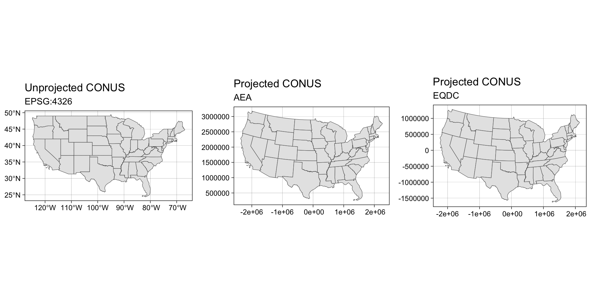
Projected Coordinate Systems (PCS)
The surface of the earth is curved but maps (and to data GIS) is flat.
Projected coordinate systems have an origin, an x axis, a y axis, and a linear unit of measure.
Going from a GCS to a PCS requires mathematical transformations.
There are three main groups of projection types:
conic:
defined by a cone touching the earth at 1 or 2 lines of tangency
best suited for mid-latitude areas
cylindrical:
defined by a cylinder touching the earth at 1 or 2 lines of tangency
best suited for large areas
planar:
defined by a plane touching the earth at 1 point or along 1 line of tangency
best suited for polar regions
Spatial Properties
All PCS distort real-world geographic features.
Think about trying to unpeel an orange while preserving the skin
The four spatial properties that are subject to distortion are: shape, area, distance and direction
A map that preserves shape is called conformal;
one that preserves area is called equal-area;
one that preserves distance is called equidistant
one that preserves direction is called azimuthal
Each map projection can preserve only one or two of the four spatial properties.
Often, projections are named after the spatial properties they preserve.
When working with small-scale (large area) maps and when multiple spatial properties are needed, it is best to break the analyses across projections to minimize errors associated with spatial distortion.
Setting CRSs/PCSs
sfc objects have two attributes to store a CRS: epsg and proj4string
datum marks the relationship between the ellipsoid and geoid
can be local (NAD27)
can be global (WGS84, NAD83)
So …
CRSs can be projected (x-y axis, measurement units (m), false origin)
All PCS are based on GCS
Projections seek to place the 3D earth on 2D
Does this by defining a plane that can be conic, cylindrical or planar
“unfolding to this plane” creates distortion of shape, area, distance, or direction
The distortion is greater from point/lines of tangency or secanacy
But …
In all cases, CRS’s place geoemtries, linked to data, on the earths surface in a way they can be related, measured, and analyzed….
Measures (GEOS Measures)
Measures are the questions we ask about the dimension of a geometry
How long is a line or polygon perimeter (unit)
What is the area of a polygon (unit2)
How far are two object from one another (unit)
Measures come from the GEOS library
Measures are in the units of the base projection
Measures can be Euclidean or geodesic
geodesic (Great Circle) distances can be more accurate by eliminating distortion
but are much slower to calculate
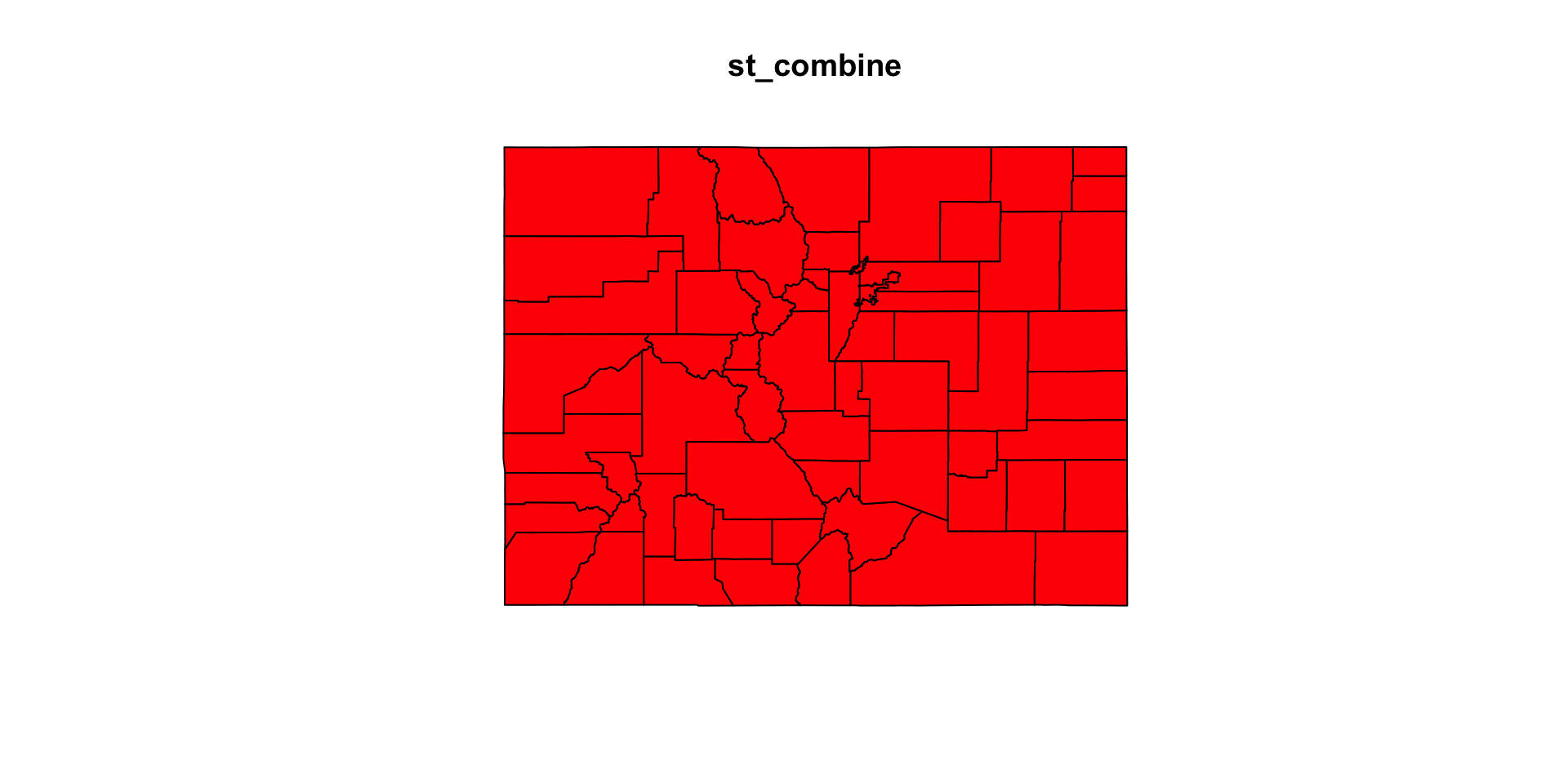
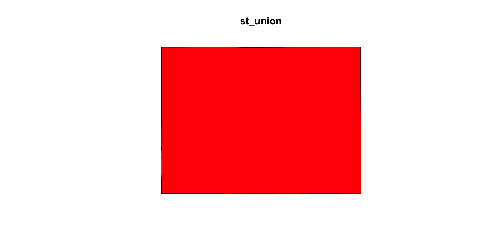
For example …
usa <-st_cast(st_union(aoi_get(state ="conus")), "MULTILINESTRING")nrow(cities)#> [1] 31254
# Great Circle Distance in GCSsystem.time({x <-st_distance(usa, cities)})# user system elapsed # 103.560 1.390 117.128 # Euclidean Distance on PCSsystem.time({x <-st_distance(usa, cities, which ="Euclidean")})# user system elapsed # 2.422 0.019 2.494
Units
When possible measure operations report results with a units appropriate for the CRS:
co <-st_read("data/co.shp")#> Reading layer `co' from data source #> `/Users/mikejohnson/github/csu-ess-330/slides/data/co.shp' #> using driver `ESRI Shapefile'#> Simple feature collection with 64 features and 4 fields#> Geometry type: MULTIPOLYGON#> Dimension: XY#> Bounding box: xmin: -109.0602 ymin: 36.99246 xmax: -102.0415 ymax: 41.00342#> Geodetic CRS: WGS 84a <-st_area(co[1,])attributes(a) |>unlist()#> units.numerator1 units.numerator2 class #> "m" "m" "units"
The units package can be used to convert between units:
units::set_units(a, km^2) # result in square kilometers#> 3062.85 [km^2]units::set_units(a, ha) # result in hectares#> 306285 [ha]
and the results can be stripped of their attributes for cases where numeric values are needed (e.g. math operators and ggplot):
The process of finding, downloading and accessing data is the first step of every analysis. Here we will go through these steps.
First go to this site and download the appropriate (free) dataset into the data directory of your project.
Once downloaded, read it into your working session using readr::read_csv() and explore the dataset until you are comfortable with the information it contains.
While this data has everything we want, it is not yet spatial. Convert the data.frame to a spatial object using st_as_sf and prescribing the coordinate variables and CRS (Hint what projection are the raw coordinates in?)
Assignment
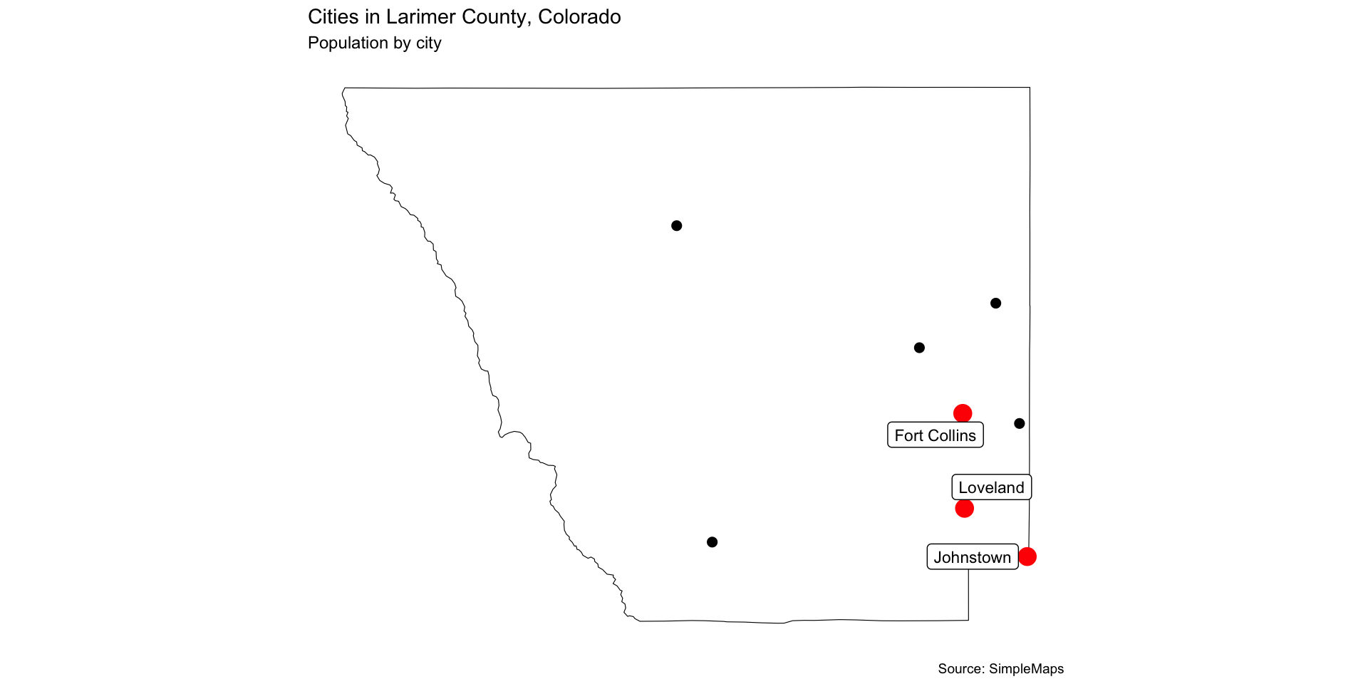
Next, we will find the county boundaries for Larimer County, Colorado. Use the aoi_get(state = "CO", county = "Larimer") function to get the county boundary.
Use st_filter to find all the cities in the dataset that are within Larimer County.
Plot the cities and the county boundary on a single map. Use geom_sf() to plot both layers and make sure to set the fill and color arguments appropriately.
Next, determine the three cities in Larimer County with the highest population and add these to the map. Use a larger point size and a different color for the points will help them stand out.
Assignment
Last, you will learn a new approach for labeling things on a ggplot that is particularly useful for cartography….
If you dont already have it, install the ggrepel package. This package provides a function called geom_label_repel() that will help you label the points without overlapping labels. The syntax is similar to geom_label() but it will automatically adjust the position of the labels to avoid overlap.
Like all ggplot2 layers, you can add this to your existing plot and first must prescribe the data to be used.
In the aesthetic mapping, you will need to specify the label argument to be the name of the city. and the geometry argument to be the geometry column of you sf object.
Finally, you need to set the stat argument to sf_coordinates so the function knows to use the coordinates of the geometry column for the label positions.
# Add labels to the cities ggrepel::geom_label_repel(data = three_largest_cities,aes(label = city, geometry = geometry),stat ="sf_coordinates",size =3)
Assignment
Your final map should look something like this (with design elements of your choosing):
Use ggsave to save your final map to the images directory of your project and submit the PNG to Canvas.