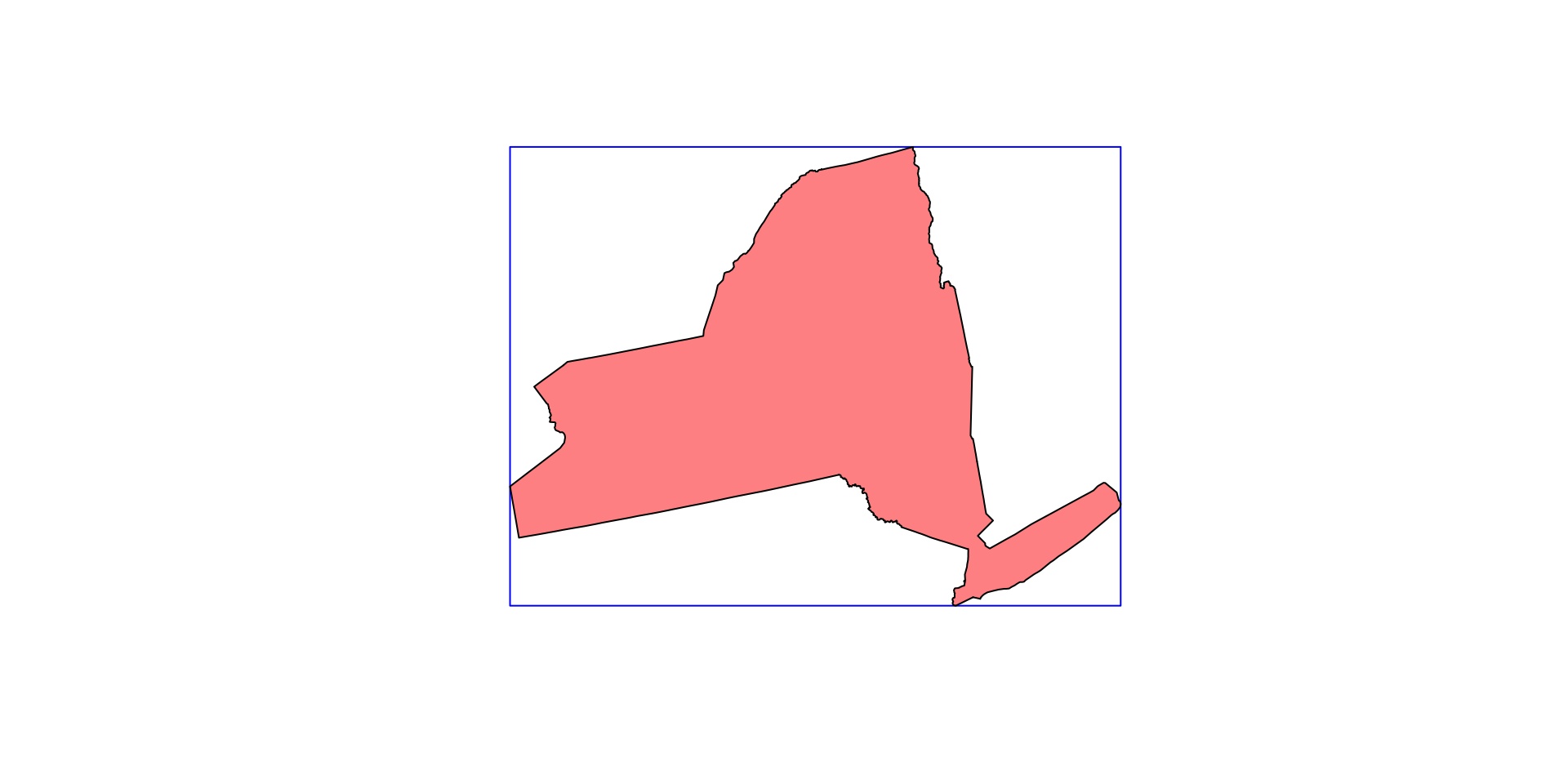
(ny <- AOI::aoi_get(state = "NY") |>
   st_transform(5070) |>
   dplyr::select(name))
#> Simple feature collection with 1 feature and 1 field
#> Geometry type: MULTIPOLYGON
#> Dimension:     XY
#> Bounding box:  xmin: 1319502 ymin: 2149150 xmax: 1997508 ymax: 2658543
#> Projected CRS: NAD83 / Conus Albers
#>       name                       geometry
#> 1 New York MULTIPOLYGON (((1661335 263...Lecture 26
Introduction to Raster Data
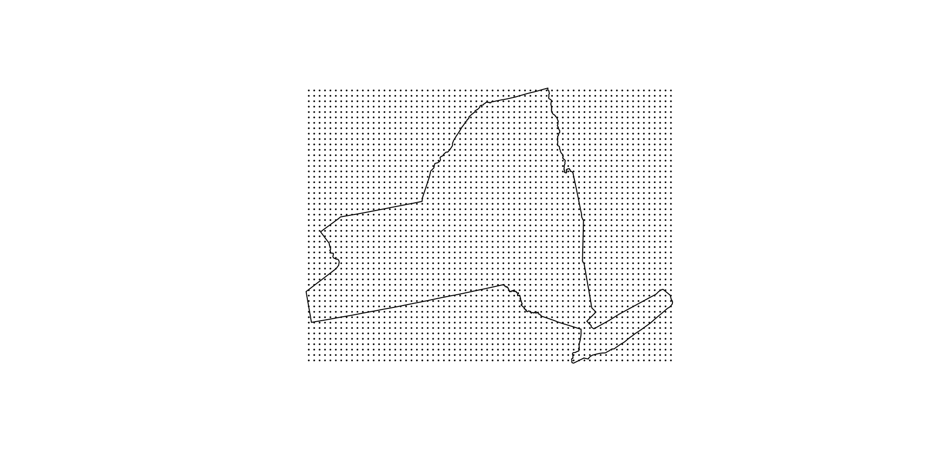
Result:
Extents can be discritized in a number of ways:
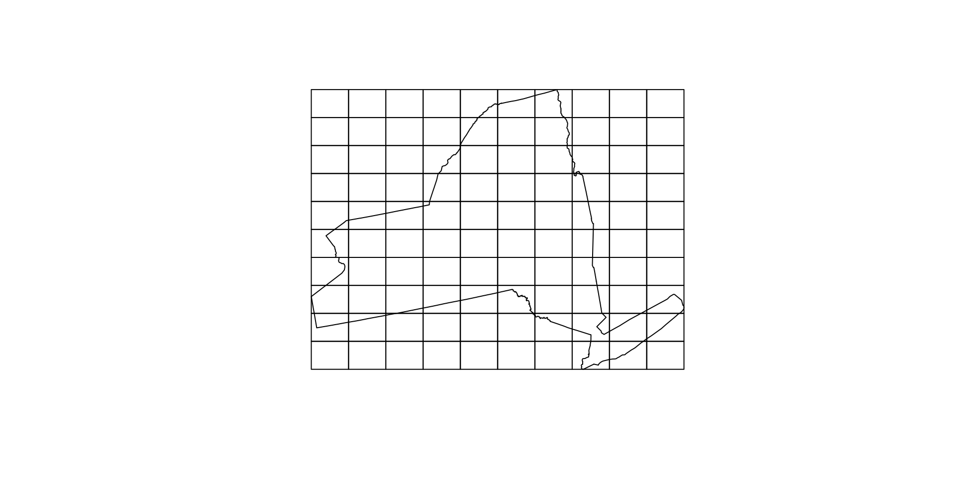
Alternative representation
Regular grids can also be indexed by their centroids
Many terms mean the same thing …
The entire raster is sometimes referred to as an “image”, “array”, “surface”, “matrix”, or “lattice” (Wise, 2000).
The all mean the same thing…
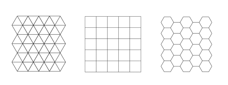
Cells of the raster are most often square, but may be rectangular (with differing resolutions in x and y directions) or other shapes that can be tessellated such as triangles and hexagons (Figure below from Peuquet, 1984).
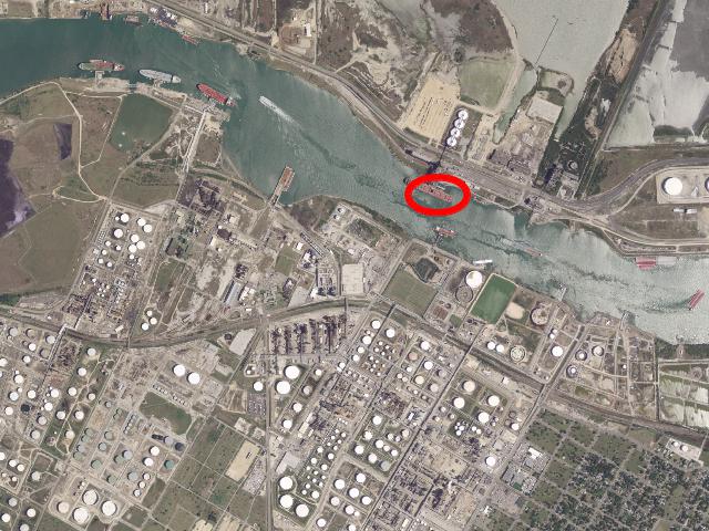
Photos and Computers …
![]()
![]()
Aerial Imagery (really just a photo 😄)

What is stored in these cells?
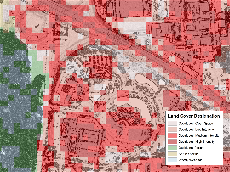
Categorical Values (integer/factor)
![]()
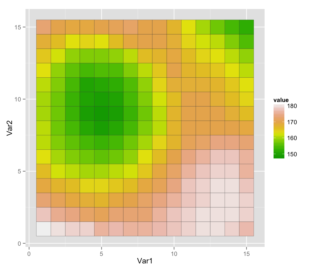
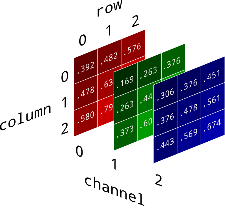
Continuous Values (numeric)
Spectral Values
- Either Color, or sensor
Why do we care?
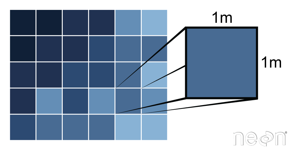
Pixels are the base unit of raster data and have a resolution
This is the X and the Y dimension of each cell in the units of the CRS
Raster images seek to discritize the real world into cell-based values
- Again either integer (categorical), continuous, or signal
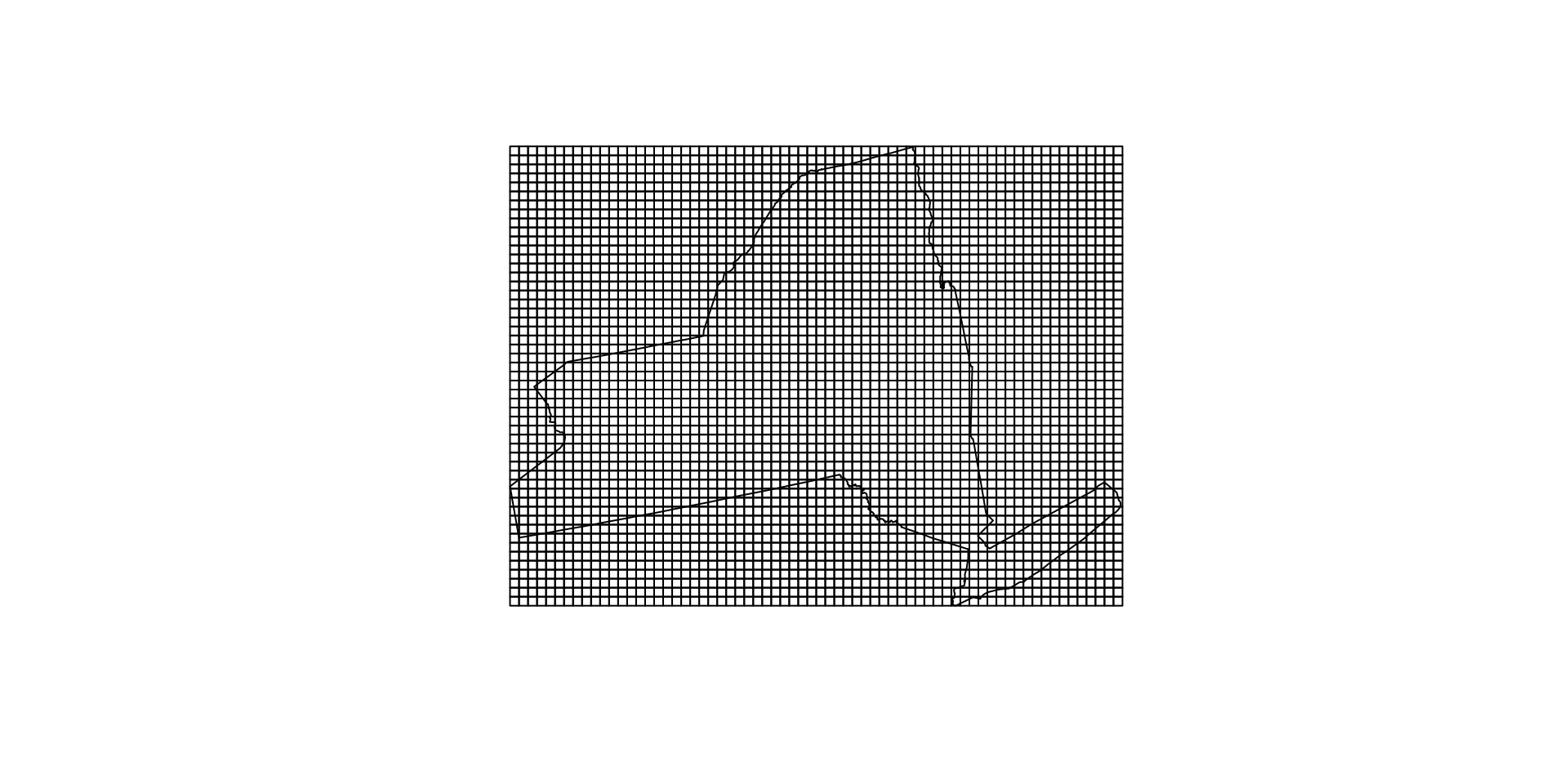
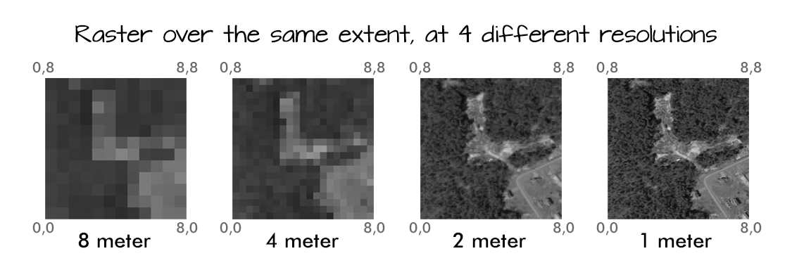
Resolution drives image clarity (granulairty)
- Higher resolution (smaller cells) = more detail, but bigger data!
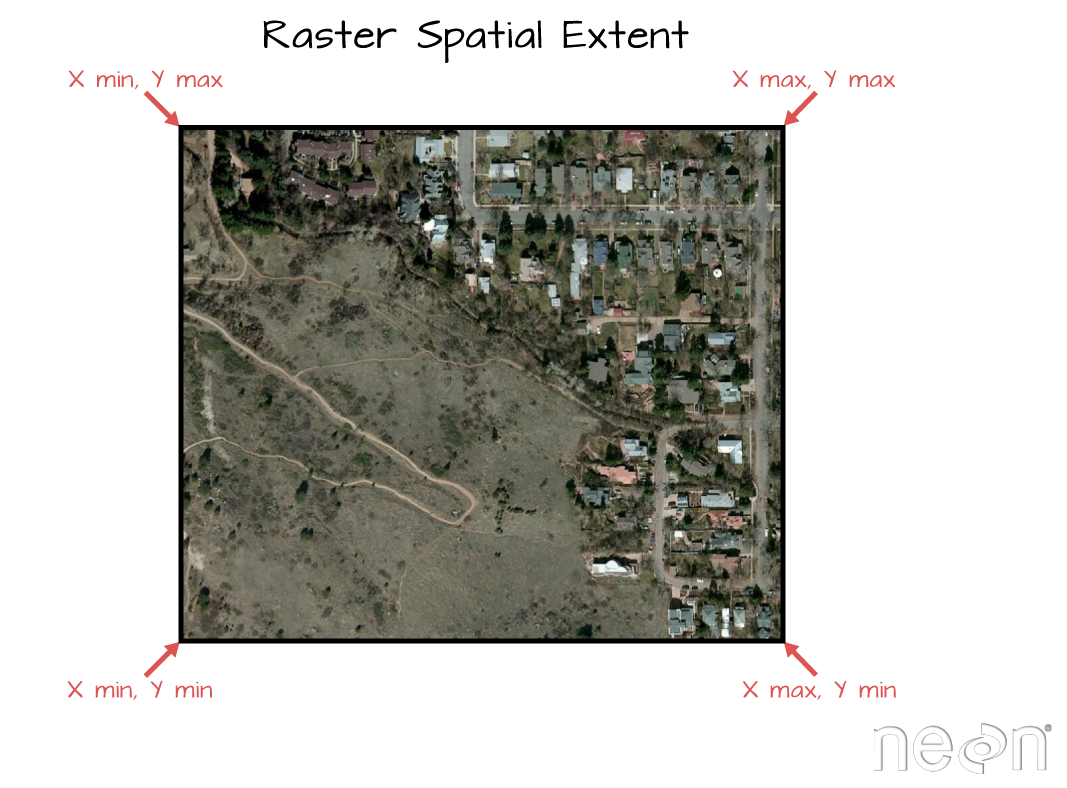
All rasters have an extent!
This is the same extent as a bounding box
Can be described as 4 values (xmin,ymin,xmax,ymax)
Implicit Coordinates
Unlike vector data, the raster data model stores the coordinate of the grid cells indirectly
Coordinates are derived from the reference (Xmin,Ymin) the resolution, and the cell index (e.g. [100,150])
For example: If we want the coordinates of a value in the 3rd row and the 40th column of a raster matrix, we have to move from the origin (Xmin, Ymin) (3 x Xres) in x-direction and (40 x Yres) in y-direction
So, any image (.png, .tif, .gif) can be read as a raster…
The raster is defined by the extent and resolution of the cells
To be spatial, the extent (thus coordinates) must be grounded in an CRS
(img = terra::rast('images/17-raster-extent.png'))
#> class       : SpatRaster
#> dimensions  : 788, 1067, 4  (nrow, ncol, nlyr)
#> resolution  : 1, 1  (x, y)
#> extent      : 0, 1067, 0, 788  (xmin, xmax, ymin, ymax)
#> coord. ref. :
#> source      : 17-raster-extent.png
#> names       : 17-rast~xtent_1, 17-rast~xtent_2, 17-rast~xtent_3, 17-rast~xtent_4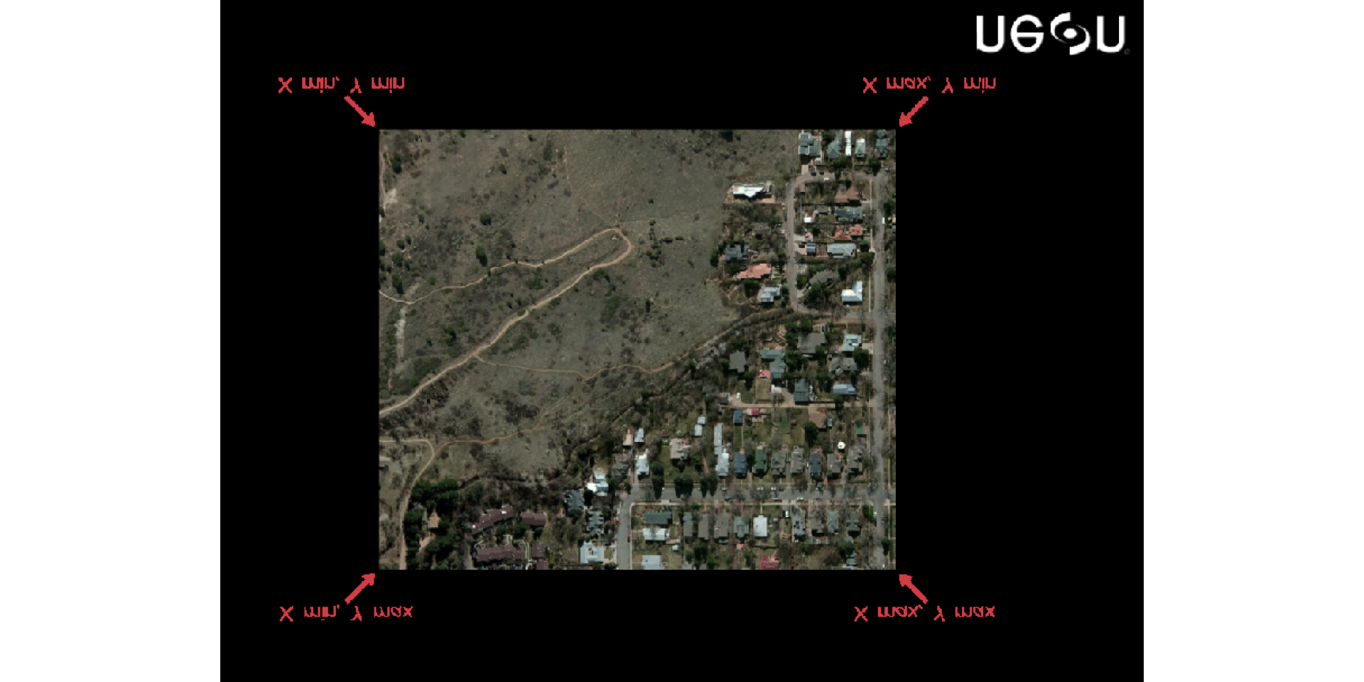
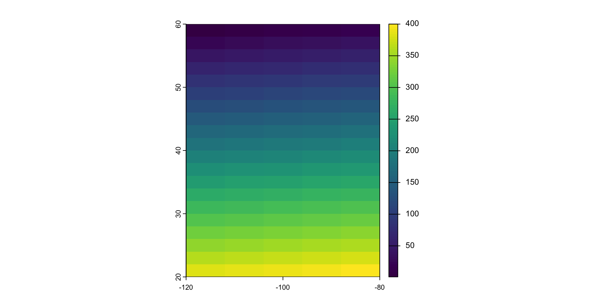
Assigning a values as a vector
values(r) <- 1:ncell(r)

r
#> class       : SpatRaster
#> dimensions  : 20, 20, 1  (nrow, ncol, nlyr)
#> resolution  : 2, 2  (x, y)
#> extent      : -120, -80, 20, 60  (xmin, xmax, ymin, ymax)
#> coord. ref. : lon/lat WGS 84 (CRS84) (OGC:CRS84)
#> source(s)   : memory
#> name        : lyr.1
#> min value   :     1
#> max value   :   400

head(values(r))
#>      lyr.1
#> [1,]     1
#> [2,]     2
#> [3,]     3
#> [4,]     4
#> [5,]     5
#> [6,]     6