Lecture 27
Raster Modification
1. Extent
When dealing with raster data, the extent is a fondational component of the raster data structure
- That is, we need to know the area the raster is covering!
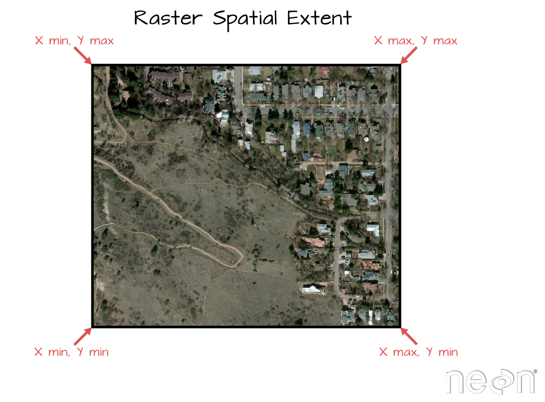
Image Source: National Ecological Observatory Network (NEON)
2. Discretization
Once we know the extent, we need to know how that space is split up
Two complimentary bit of information can tell us this:
- Resolution (res)
- Number of row and number of columns (nrow/ncol)
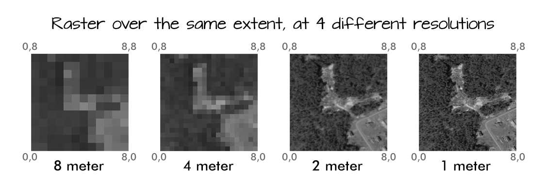
Image Source: National Ecological Observatory Network (NEON)
Find elevation data for Fort Collins:
- Define the AOI
- Read data from elevation map tiles, for a specific zoom, and crop to the AOI
- The resulting raster …
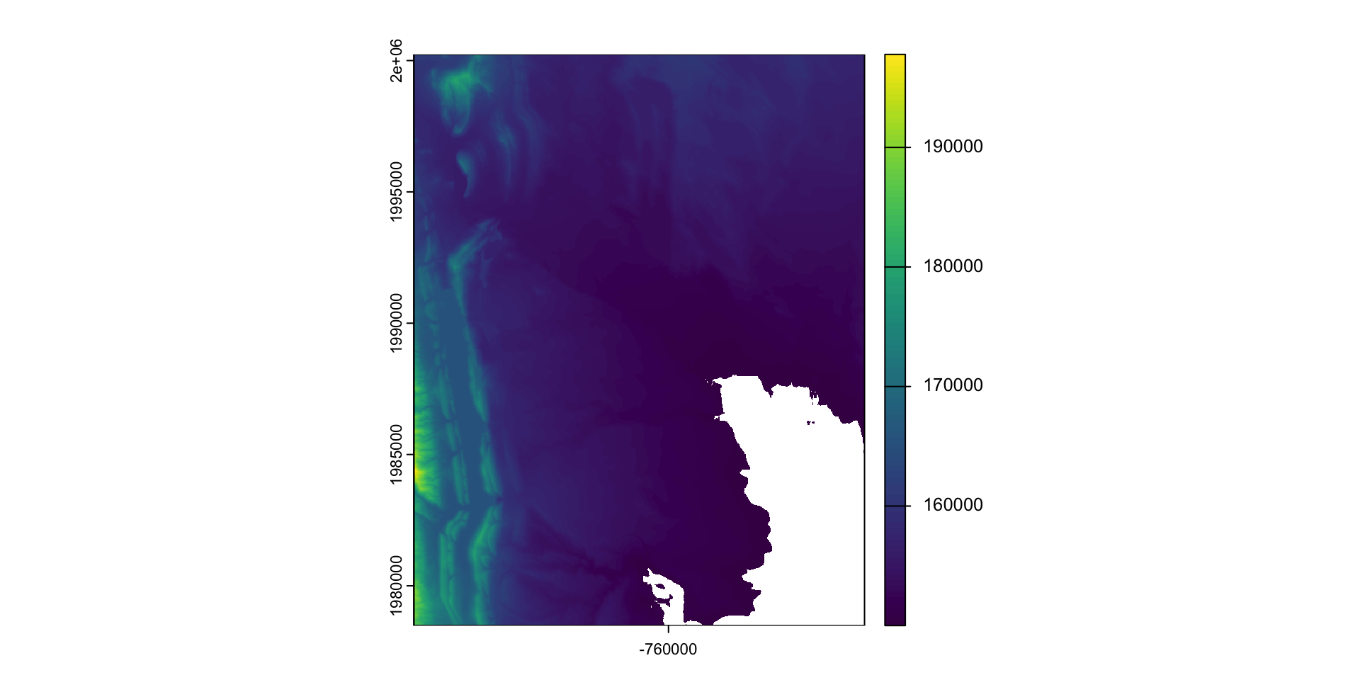
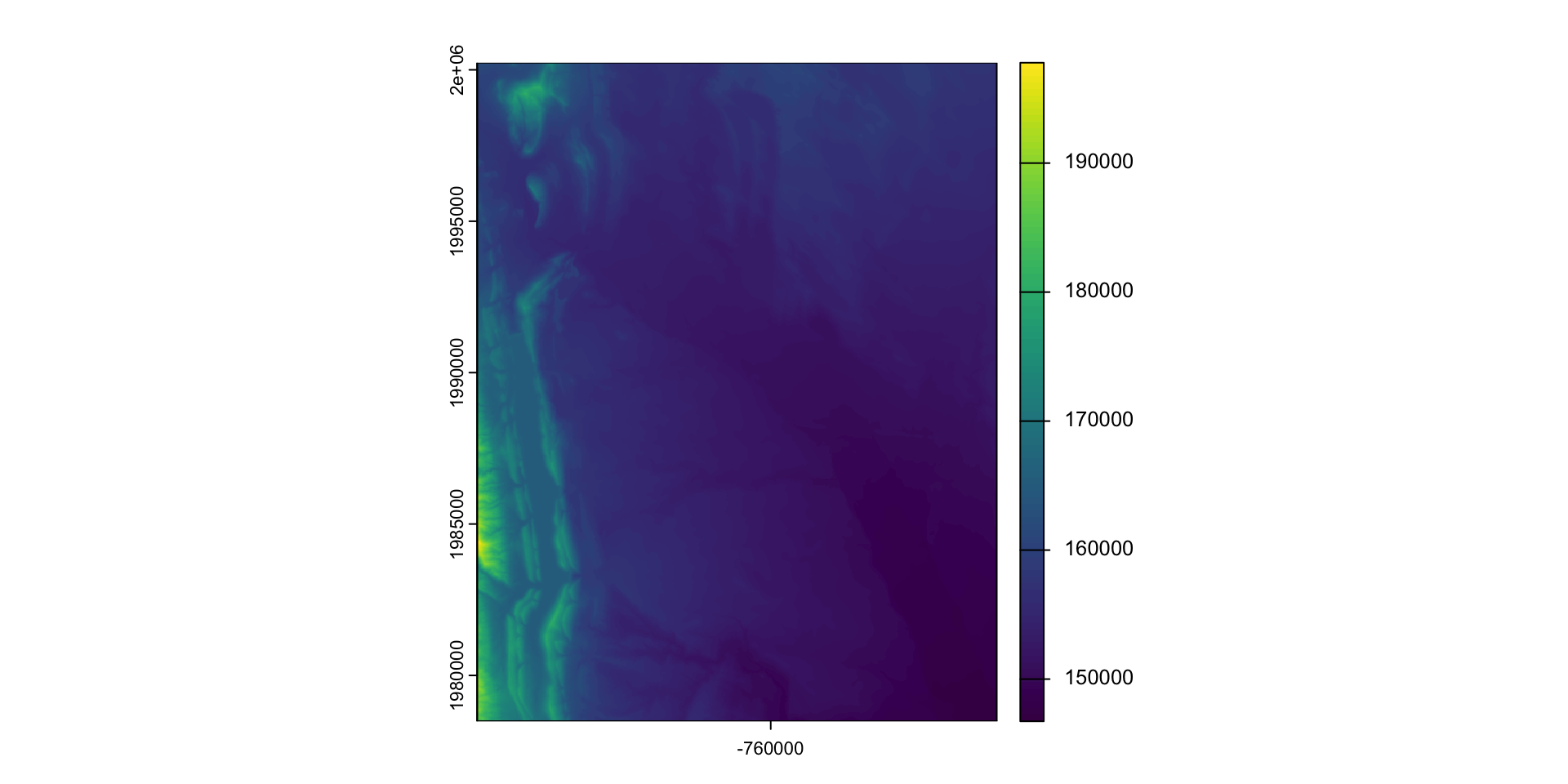
(elev = rast("data/foco-elev.tif"))
#> class       : SpatRaster
#> dimensions  : 725, 572, 1  (nrow, ncol, nlyr)
#> resolution  : 30, 30  (x, y)
#> extent      : -769695, -752535, 1978485, 2000235  (xmin, xmax, ymin, ymax)
#> coord. ref. : +proj=aea +lat_0=23 +lon_0=-96 +lat_1=29.5 +lat_2=45.5 +x_0=0 +y_0=0 +datum=NAD83 +units=m +no_defs
#> source      : foco-elev.tif
#> name        :    dem
#> min value   : 146730
#> max value   : 197781
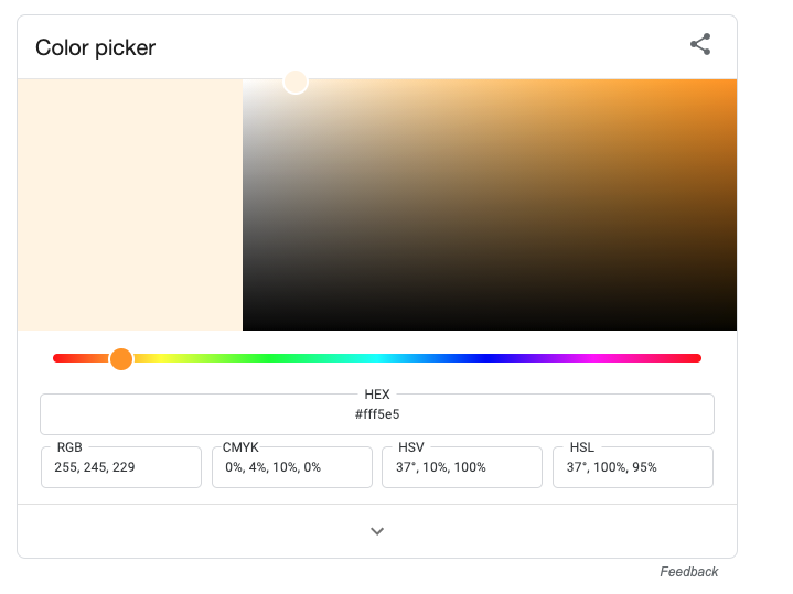
Google Color Picker
Replacement
- Raster values can be replaced on a conditional statements
- Doing this changes the underlying data!
- If you want to retain the original data, you must make a copy of the base layer

Modifying a raster
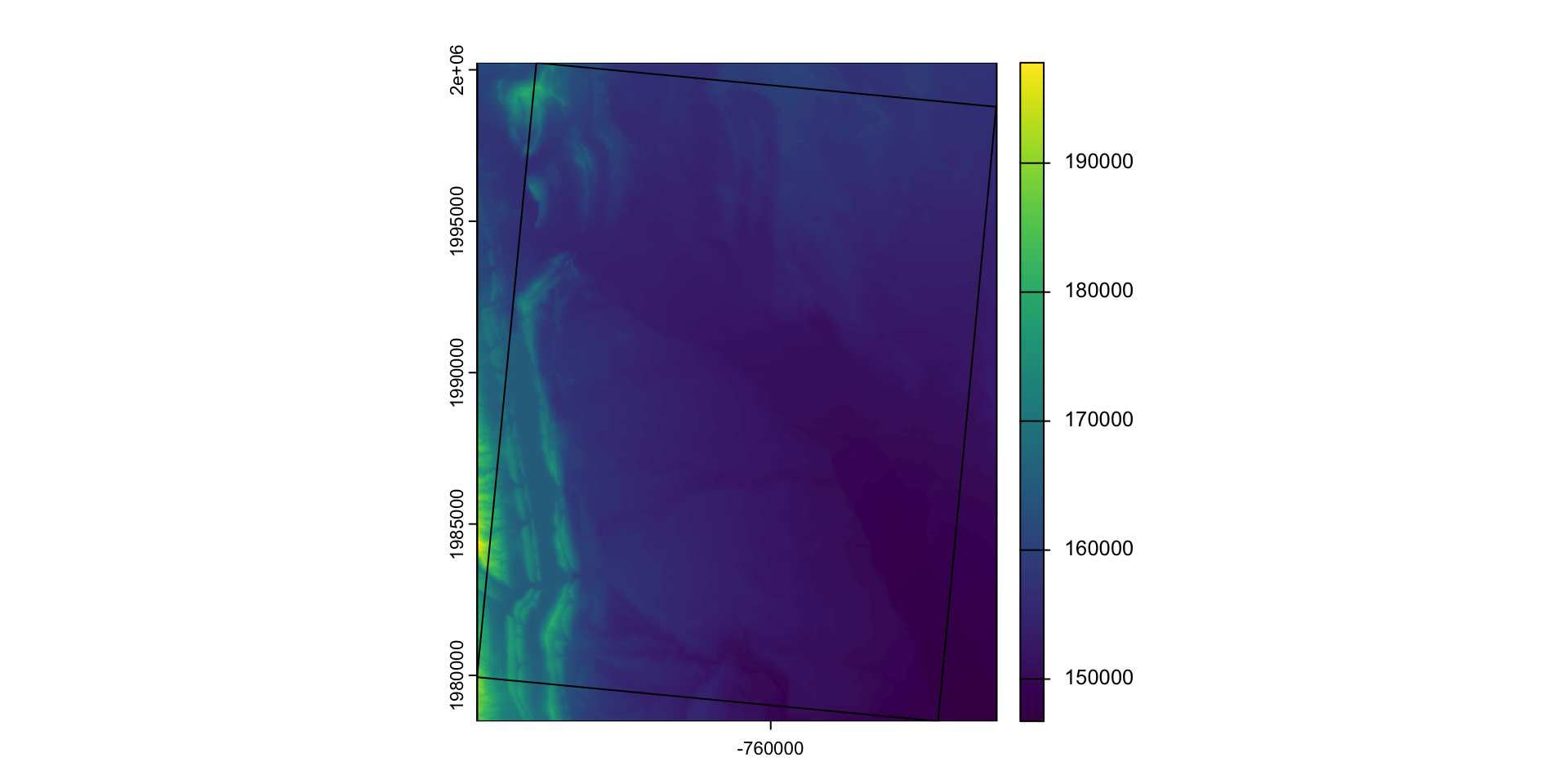
When we want to modify the extent of a raster we can clip it to a new bounds
crop: lets you reduce the extent of a raster to the extent of another, overlapping object:

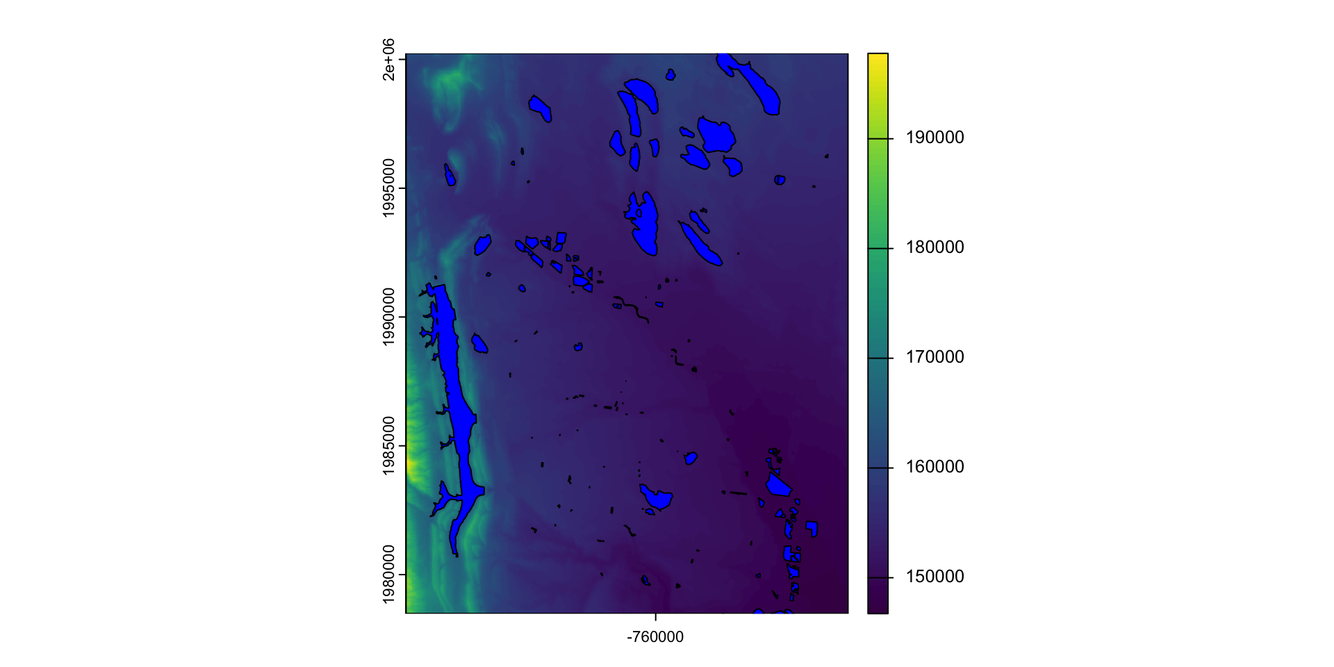
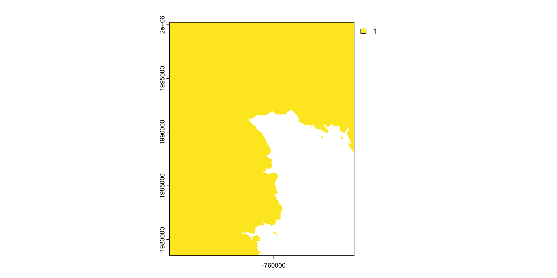
What is mask doing?

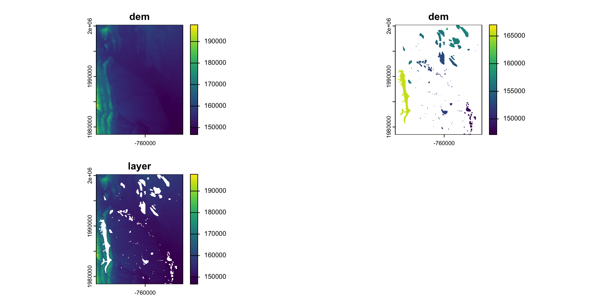
Crop or/and mask
- Crop is more efficient then mask
- Often you will want to mask and crop a raster
- The correct way to do this is crop then mask

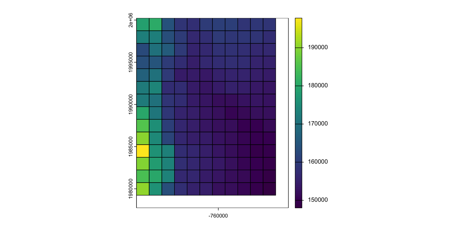
Aggregate and disaggregate
aggregateanddisaggregateallow for changing the resolution of a Raster object.This is similar to the zoom scaling on a web map except the scale factor is not set to 2
For aggregate, you need to specify a function determining what to do with the grouped cell values (default = mean).

app
Just like a vector, we can apply functions over a raster with
appThese types of formulas are very useful for thresholding analysis
These types of functions are very simular in concept to
map_*
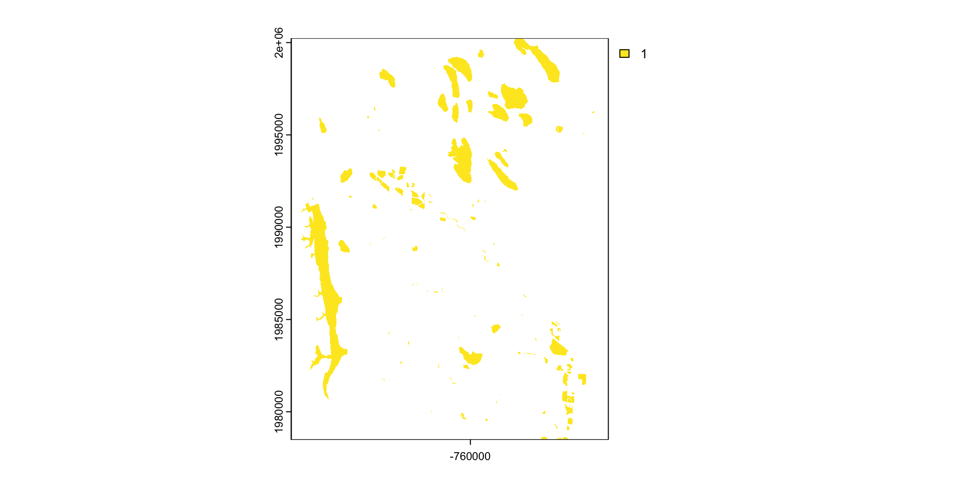
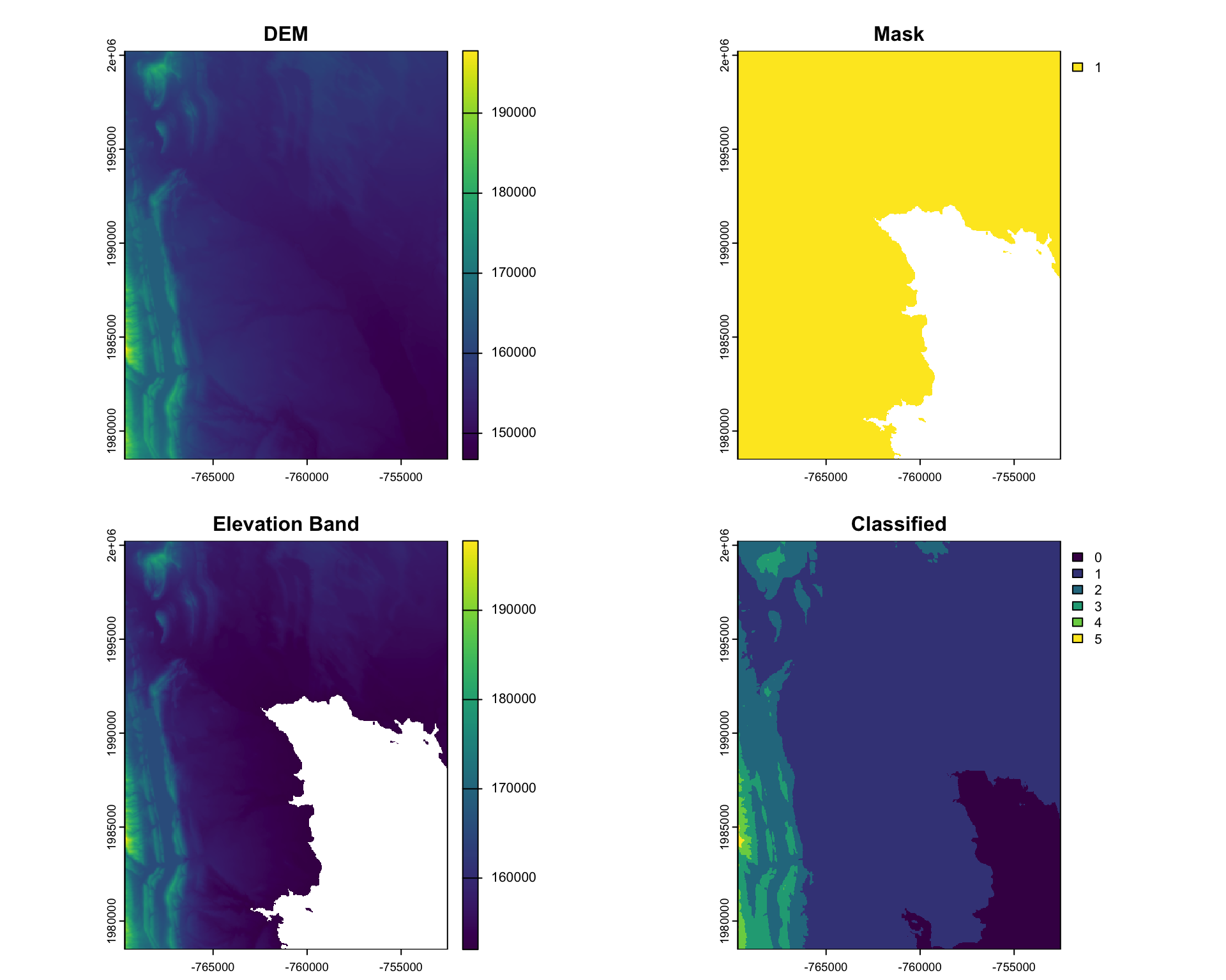
Question: separate Fort Collins into the higher and lower elevations
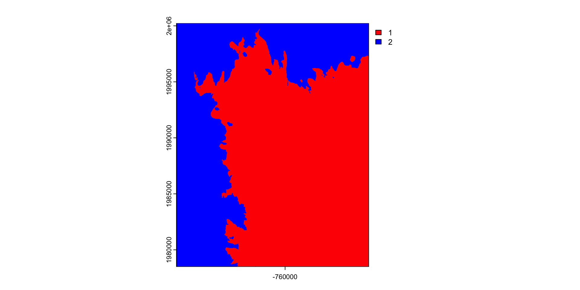
Results
Multiply cell-wise
- algebraic, logical, and functional operations act on a raster cell-wise

Plot

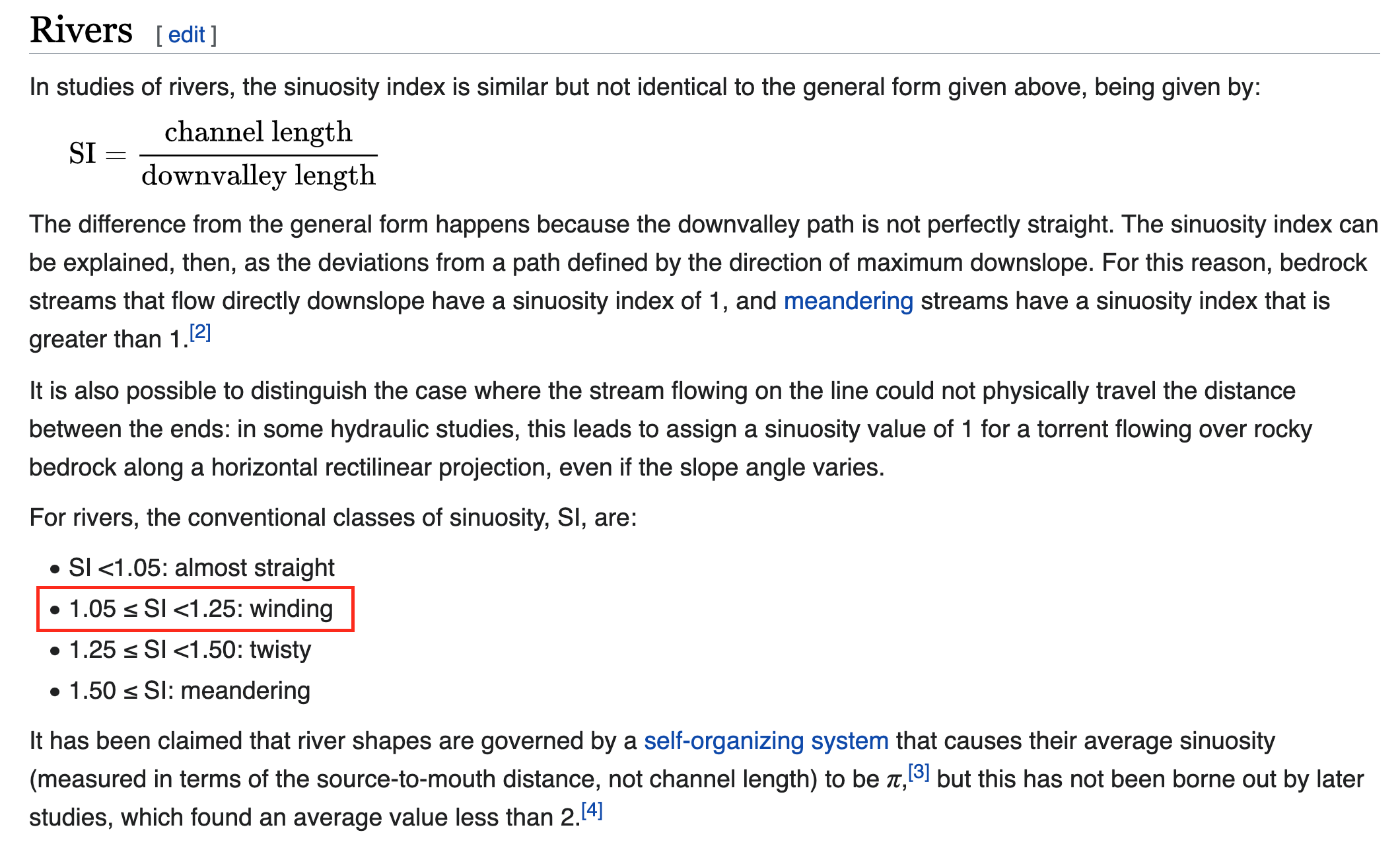
Lets find the longest river segment IN our extent


Computation 1: Sinuosity
Channel sinuosity is calculated by dividing the length of the stream channel by the straight line distance between the end points of the selected channel reach.
Computation 3: River Profile
The river profile is the elevation of the river at each point along the river.
