Lecture 03

Data Types & Projects

Mike Johnson

mike.johnson@colostate.edu

2025-02-09

Slido!

Important

If you are having trouble setting up R, RStudio, ect email the teaching team ASAP!

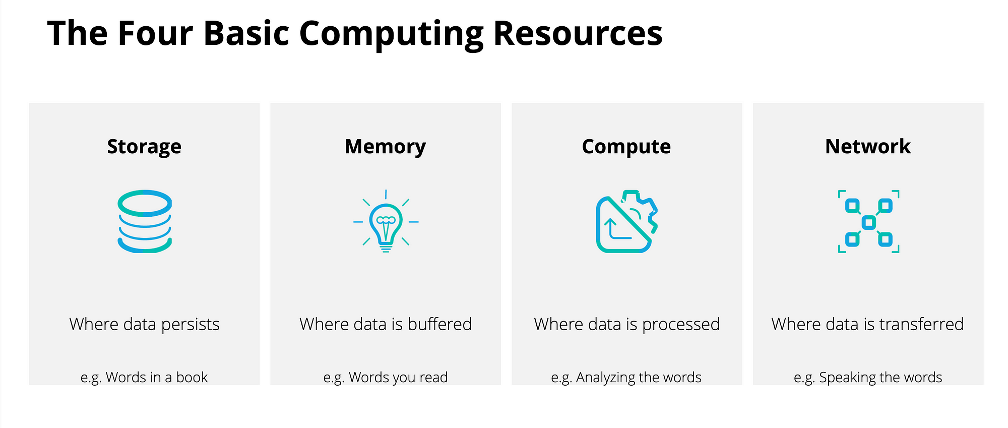
Back to Compute:

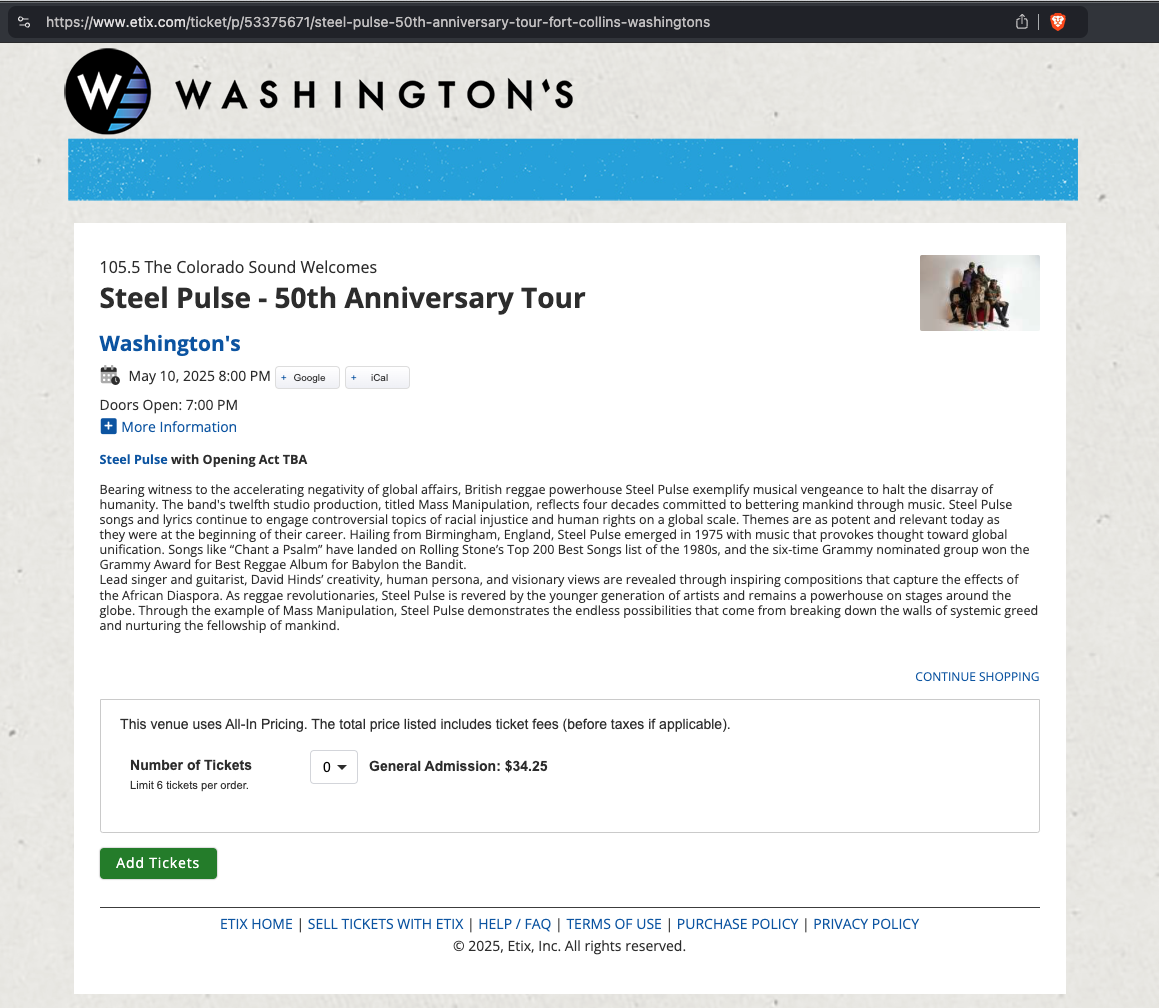
Information

https://www.etix.com/ticket/p/53375671/steel-pulse-50th-anniversary-tour-fort-collins-washingtons

Important

index.html is everywhere online (lets take a look!)

I/O

Input and Output

• I/O stands for Input/Output
• It provides the guideline for how to read bytes, stored as a file, at a specific path
• Languages (like R) have readers that take general directions (e.g. “0x89 0x50” is how a PNG file starts.) and interprets it to how the language needs the data

Read from Disk

img <- png::readPNG('images/03-bit-byte.png')

Return from Server: JSON

'https://geoconnex.us/ref/mainstems/352913' |> 
1 jsonlite::fromJSON()
$type
[1] "Feature"

$properties
$properties$head_nhdpv2_comid
[1] "https://geoconnex.us/nhdplusv2/comid/2902889"

$properties$head_nhdpv1_comid
NULL

$properties$fid
[1] 18032

$properties$outlet_nhdpv2_comid
[1] "https://geoconnex.us/nhdplusv2/comid/2903809"

$properties$outlet_nhdpv1_comid
NULL

$properties$uri
[1] "https://geoconnex.us/ref/mainstems/352913"

$properties$head_nhdpv2huc12
[1] "https://geoconnex.us/nhdplusv2/huc12/101900070202"

$properties$head_2020huc12
[1] "101900070202"

$properties$featuretype
[1] "['https://www.opengis.net/def/schema/hy_features/hyf/HY_FlowPath', 'https://www.opengis.net/def/schema/hy_features/hyf/HY_WaterBody']"

$properties$outlet_nhdpv2huc12
[1] "https://geoconnex.us/nhdplusv2/huc12/101900071008"

$properties$outlet_2020huc12
[1] "101900071008"

$properties$downstream_mainstem_id
[1] "https://geoconnex.us/ref/mainstems/313255"

$properties$lengthkm
[1] 200.5

$properties$superseded
[1] FALSE

$properties$encompassing_mainstem_basins
[1] "['https://geoconnex.us/ref/mainstems/313255', 'https://geoconnex.us/ref/mainstems/312532', 'https://geoconnex.us/ref/mainstems/312091']"

$properties$outlet_drainagearea_sqkm
[1] 4875.9

$properties$new_mainstemid
[1] ""

$properties$name_at_outlet
[1] "Cache la Poudre River"

$properties$head_rf1id
[1] 22904

$properties$name_at_outlet_gnis_id
[1] 205018

$properties$outlet_rf1id
[1] 22867

$properties$datasets
                                                       monitoringLocation
1 https://sta.geoconnex.dev/collections/USGS/Things/items/'USGS-06752280'
2 https://sta.geoconnex.dev/collections/USGS/Things/items/'USGS-06752280'
3 https://sta.geoconnex.dev/collections/USGS/Things/items/'USGS-06752280'
4 https://sta.geoconnex.dev/collections/USGS/Things/items/'USGS-06752280'
       siteName                                           datasetDescription
1 USGS-06752280 Gage height / USGS-06752280-7176ea9161f94cbf8bd7b30aba7891fd
2 USGS-06752280 Gage height / USGS-06752280-7176ea9161f94cbf8bd7b30aba7891fd
3 USGS-06752280   Discharge / USGS-06752280-b9cc8727355d4de08f7c0826530c96ce
4 USGS-06752280   Discharge / USGS-06752280-b9cc8727355d4de08f7c0826530c96ce
    type
1 Stream
2 Stream
3 Stream
4 Stream
                                                                           url
1 https://waterdata.usgs.gov/monitoring-location/06752280/#parameterCode=00065
2 https://waterdata.usgs.gov/monitoring-location/06752280/#parameterCode=00065
3 https://waterdata.usgs.gov/monitoring-location/06752280/#parameterCode=00060
4 https://waterdata.usgs.gov/monitoring-location/06752280/#parameterCode=00060
                                              variableMeasured variableUnit
1 Gage height / USGS-06752280-7176ea9161f94cbf8bd7b30aba7891fd           ft
2 Gage height / USGS-06752280-7176ea9161f94cbf8bd7b30aba7891fd           ft
3   Discharge / USGS-06752280-b9cc8727355d4de08f7c0826530c96ce       ft^3/s
4   Discharge / USGS-06752280-b9cc8727355d4de08f7c0826530c96ce       ft^3/s
  measurementTechnique                          temporalCoverage
1          observation 2024-08-30T09:15:00Z/2024-09-09T18:00:00Z
2          observation 2024-08-30T09:15:00Z/2024-09-09T18:00:00Z
3          observation 2024-08-30T09:15:00Z/2024-09-09T18:00:00Z
4          observation 2024-08-30T09:15:00Z/2024-09-09T18:00:00Z
                   distributionName
1 USGS Instantaneous Values Service
2             USGS SensorThings API
3             USGS SensorThings API
4 USGS Instantaneous Values Service
                                                                                                      distributionURL
1                                https://waterservices.usgs.gov/nwis/iv/?sites=USGS:06752280¶meterCd=00065&format=rdb
2 https://labs.waterdata.usgs.gov/sta/v1.1/Datastreams('7176ea9161f94cbf8bd7b30aba7891fd')?$expand=Thing,Observations
3 https://labs.waterdata.usgs.gov/sta/v1.1/Datastreams('b9cc8727355d4de08f7c0826530c96ce')?$expand=Thing,Observations
4                                https://waterservices.usgs.gov/nwis/iv/?sites=USGS:06752280¶meterCd=00060&format=rdb
         distributionFormat                                        wkt
1 text/tab-separated-values POINT (-105.011365078564 40.5519269209862)
2          application/json POINT (-105.011365078564 40.5519269209862)
3          application/json POINT (-105.011365078564 40.5519269209862)
4 text/tab-separated-values POINT (-105.011365078564 40.5519269209862)


$id
[1] "352913"

$geometry
$geometry$type
[1] "LineString"

$geometry$coordinates
            [,1]     [,2]
  [1,] -105.8107 40.42002
  [2,] -105.7947 40.43621
  [3,] -105.7852 40.44236
  [4,] -105.7735 40.44730
  [5,] -105.7606 40.45680
  [6,] -105.7513 40.46771
  [7,] -105.7444 40.46977
  [8,] -105.7345 40.46944
  [9,] -105.7318 40.47216
 [10,] -105.7320 40.47614
 [11,] -105.7383 40.48742
 [12,] -105.7356 40.49914
 [13,] -105.7376 40.50436
 [14,] -105.7371 40.51262
 [15,] -105.7421 40.51571
 [16,] -105.7427 40.51838
 [17,] -105.7473 40.52252
 [18,] -105.7499 40.53037
 [19,] -105.7526 40.53142
 [20,] -105.7547 40.54133
 [21,] -105.7642 40.54846
 [22,] -105.7739 40.55154
 [23,] -105.7793 40.55726
 [24,] -105.7907 40.56379
 [25,] -105.7984 40.57411
 [26,] -105.8025 40.57606
 [27,] -105.8041 40.58197
 [28,] -105.8016 40.58544
 [29,] -105.8042 40.58956
 [30,] -105.8044 40.59581
 [31,] -105.8002 40.59709
 [32,] -105.7954 40.61033
 [33,] -105.8007 40.61327
 [34,] -105.7993 40.61670
 [35,] -105.8005 40.62526
 [36,] -105.8074 40.63057
 [37,] -105.8062 40.63652
 [38,] -105.8094 40.64254
 [39,] -105.8102 40.65254
 [40,] -105.8129 40.65833
 [41,] -105.8092 40.66116
 [42,] -105.8092 40.66420
 [43,] -105.8039 40.67100
 [44,] -105.7970 40.66987
 [45,] -105.7869 40.67158
 [46,] -105.7764 40.67752
 [47,] -105.7662 40.68802
 [48,] -105.7609 40.69060
 [49,] -105.7587 40.69469
 [50,] -105.7591 40.69991
 [51,] -105.7544 40.70198
 [52,] -105.7538 40.70562
 [53,] -105.7495 40.70701
 [54,] -105.7511 40.70825
 [55,] -105.7461 40.71049
 [56,] -105.7413 40.71027
 [57,] -105.7398 40.71210
 [58,] -105.7374 40.71162
 [59,] -105.7328 40.71387
 [60,] -105.7276 40.71037
 [61,] -105.7253 40.70610
 [62,] -105.7217 40.70688
 [63,] -105.7159 40.70043
 [64,] -105.7073 40.69936
 [65,] -105.7065 40.70083
 [66,] -105.7040 40.69795
 [67,] -105.7013 40.69703
 [68,] -105.6996 40.69859
 [69,] -105.6936 40.69502
 [70,] -105.6871 40.69732
 [71,] -105.6797 40.69380
 [72,] -105.6768 40.69444
 [73,] -105.6742 40.69835
 [74,] -105.6679 40.69730
 [75,] -105.6624 40.70014
 [76,] -105.6502 40.70014
 [77,] -105.6355 40.70280
 [78,] -105.6274 40.70070
 [79,] -105.6243 40.69759
 [80,] -105.6196 40.69807
 [81,] -105.6063 40.69424
 [82,] -105.5992 40.69751
 [83,] -105.5818 40.69733
 [84,] -105.5772 40.69893
 [85,] -105.5740 40.69819
 [86,] -105.5670 40.70100
 [87,] -105.5621 40.69892
 [88,] -105.5538 40.70022
 [89,] -105.5386 40.69987
 [90,] -105.5309 40.69817
 [91,] -105.5227 40.69891
 [92,] -105.5191 40.69726
 [93,] -105.5195 40.69516
 [94,] -105.5158 40.69154
 [95,] -105.5127 40.69170
 [96,] -105.5087 40.68952
 [97,] -105.5027 40.69180
 [98,] -105.4943 40.69020
 [99,] -105.4913 40.68810
[100,] -105.4885 40.69046
[101,] -105.4862 40.68865
[102,] -105.4802 40.67479
[103,] -105.4777 40.67390
[104,] -105.4728 40.67521
[105,] -105.4713 40.68141
[106,] -105.4670 40.68325
[107,] -105.4625 40.68311
[108,] -105.4582 40.68012
[109,] -105.4553 40.68033
[110,] -105.4530 40.68326
[111,] -105.4468 40.68624
[112,] -105.4505 40.69434
[113,] -105.4450 40.69480
[114,] -105.4417 40.69748
[115,] -105.4347 40.69396
[116,] -105.4325 40.69073
[117,] -105.4357 40.68084
[118,] -105.4303 40.67707
[119,] -105.4292 40.67449
[120,] -105.4231 40.67671
[121,] -105.4180 40.67383
[122,] -105.4113 40.67884
[123,] -105.4123 40.68166
[124,] -105.4092 40.68392
[125,] -105.4039 40.68273
[126,] -105.3965 40.68457
[127,] -105.3940 40.68292
[128,] -105.3899 40.68285
[129,] -105.3880 40.68532
[130,] -105.3816 40.68358
[131,] -105.3769 40.68784
[132,] -105.3792 40.69168
[133,] -105.3766 40.69464
[134,] -105.3705 40.69230
[135,] -105.3717 40.68951
[136,] -105.3684 40.68727
[137,] -105.3627 40.68859
[138,] -105.3552 40.68820
[139,] -105.3455 40.69111
[140,] -105.3413 40.69072
[141,] -105.3368 40.69413
[142,] -105.3330 40.69310
[143,] -105.3294 40.69476
[144,] -105.3228 40.68948
[145,] -105.2996 40.68690
[146,] -105.2978 40.68990
[147,] -105.2954 40.68873
[148,] -105.2879 40.69014
[149,] -105.2888 40.69415
[150,] -105.2813 40.69588
[151,] -105.2804 40.69867
[152,] -105.2716 40.69608
[153,] -105.2646 40.69751
[154,] -105.2648 40.69298
[155,] -105.2553 40.69178
[156,] -105.2557 40.69766
[157,] -105.2458 40.70302
[158,] -105.2424 40.70346
[159,] -105.2411 40.70142
[160,] -105.2466 40.69878
[161,] -105.2420 40.69565
[162,] -105.2390 40.69067
[163,] -105.2363 40.69083
[164,] -105.2354 40.68902
[165,] -105.2367 40.68673
[166,] -105.2403 40.68598
[167,] -105.2364 40.68348
[168,] -105.2380 40.67122
[169,] -105.2326 40.66894
[170,] -105.2290 40.67203
[171,] -105.2251 40.66455
[172,] -105.2128 40.66273
[173,] -105.2109 40.65982
[174,] -105.2044 40.65926
[175,] -105.2016 40.66088
[176,] -105.1860 40.65664
[177,] -105.1738 40.64820
[178,] -105.1729 40.64195
[179,] -105.1678 40.63680
[180,] -105.1686 40.63163
[181,] -105.1667 40.62971
[182,] -105.1435 40.62473
[183,] -105.1390 40.62070
[184,] -105.1281 40.61912
[185,] -105.1206 40.61313
[186,] -105.1159 40.61411
[187,] -105.1136 40.61180
[188,] -105.1069 40.61210
[189,] -105.1033 40.60709
[190,] -105.0987 40.60443
[191,] -105.0926 40.60143
[192,] -105.0798 40.59838
[193,] -105.0712 40.59158
[194,] -105.0679 40.59177
[195,] -105.0696 40.58813
[196,] -105.0656 40.58710
[197,] -105.0656 40.58408
[198,] -105.0594 40.58332
[199,] -105.0582 40.58048
[200,] -105.0525 40.57981
[201,] -105.0481 40.57612
[202,] -105.0447 40.57850
[203,] -105.0351 40.57859
[204,] -105.0323 40.57250
[205,] -105.0279 40.57130
[206,] -105.0269 40.56611
[207,] -105.0229 40.56038
[208,] -105.0191 40.55860
[209,] -105.0169 40.55285
[210,] -105.0137 40.55081
[211,] -105.0093 40.55136
[212,] -105.0073 40.54840
[213,] -105.0025 40.54920
[214,] -104.9973 40.54249
[215,] -104.9995 40.53741
[216,] -104.9945 40.53128
[217,] -104.9892 40.53326
[218,] -104.9860 40.53086
[219,] -104.9858 40.52191
[220,] -104.9807 40.52148
[221,] -104.9808 40.51494
[222,] -104.9764 40.51622
[223,] -104.9748 40.50222
[224,] -104.9732 40.50117
[225,] -104.9704 40.50311
[226,] -104.9675 40.50229
[227,] -104.9680 40.49907
[228,] -104.9644 40.49724
[229,] -104.9677 40.49476
[230,] -104.9650 40.49072
[231,] -104.9662 40.48838
[232,] -104.9583 40.48550
[233,] -104.9575 40.48022
[234,] -104.9527 40.47862
[235,] -104.9506 40.47546
[236,] -104.9467 40.47604
[237,] -104.9417 40.47053
[238,] -104.9385 40.46998
[239,] -104.9373 40.47183
[240,] -104.9344 40.46961
[241,] -104.9303 40.46911
[242,] -104.9289 40.46660
[243,] -104.9242 40.46404
[244,] -104.9192 40.46395
[245,] -104.9208 40.46722
[246,] -104.9188 40.46932
[247,] -104.9168 40.46907
[248,] -104.9130 40.46475
[249,] -104.9163 40.46173
[250,] -104.9153 40.45967
[251,] -104.9106 40.46242
[252,] -104.9064 40.46281
[253,] -104.9054 40.45537
[254,] -104.9015 40.45528
[255,] -104.8977 40.45320
[256,] -104.8940 40.45505
[257,] -104.8897 40.44803
[258,] -104.8840 40.44647
[259,] -104.8836 40.44336
[260,] -104.8795 40.44148
[261,] -104.8765 40.44201
[262,] -104.8760 40.44020
[263,] -104.8783 40.43780
[264,] -104.8771 40.43647
[265,] -104.8736 40.43697
[266,] -104.8706 40.43997
[267,] -104.8670 40.44100
[268,] -104.8657 40.44530
[269,] -104.8625 40.44450
[270,] -104.8593 40.43926
[271,] -104.8539 40.44278
[272,] -104.8505 40.44132
[273,] -104.8477 40.44310
[274,] -104.8442 40.44310
[275,] -104.8386 40.44738
[276,] -104.8341 40.44445
[277,] -104.8313 40.44438
[278,] -104.8309 40.44758
[279,] -104.8279 40.44834
[280,] -104.8132 40.44666
[281,] -104.8076 40.44217
[282,] -104.8042 40.44526
[283,] -104.8009 40.44288
[284,] -104.7965 40.44429
[285,] -104.7999 40.44693
[286,] -104.7988 40.44853
[287,] -104.7875 40.44419
[288,] -104.7842 40.44701
[289,] -104.7800 40.44666
[290,] -104.7775 40.44821
[291,] -104.7760 40.44775
[292,] -104.7767 40.44547
[293,] -104.7734 40.44601
[294,] -104.7667 40.44012
[295,] -104.7652 40.44076
[296,] -104.7653 40.44383
[297,] -104.7676 40.44825
[298,] -104.7630 40.44772
[299,] -104.7627 40.44493
[300,] -104.7601 40.44433
[301,] -104.7554 40.45126
[302,] -104.7429 40.45225
[303,] -104.7305 40.44885
[304,] -104.7221 40.44988
[305,] -104.7175 40.44765
[306,] -104.7172 40.44522
[307,] -104.7116 40.44582
[308,] -104.7109 40.44188
[309,] -104.7063 40.44100
[310,] -104.7008 40.44235
[311,] -104.6966 40.44093
[312,] -104.6878 40.44075
[313,] -104.6887 40.43744
[314,] -104.6861 40.43277
[315,] -104.6829 40.42996
[316,] -104.6801 40.42382
[317,] -104.6739 40.41975
[318,] -104.6710 40.42220
[319,] -104.6665 40.42262
[320,] -104.6607 40.42054
[321,] -104.6518 40.42036
[322,] -104.6480 40.42162
[323,] -104.6396 40.41798
[324,] -104.6331 40.41999
[325,] -104.6293 40.41867
[326,] -104.6225 40.42214
[327,] -104.6195 40.41965
[328,] -104.6173 40.42244
[329,] -104.6091 40.42322
[330,] -104.6075 40.42535
[331,] -104.6022 40.42493
[332,] -104.6000 40.42158


$prev
[1] "352803"

$`next`
[1] "352986"

$links
                  type        rel                                   title
1     application/json       root The landing page of this server as JSON
2            text/html       root The landing page of this server as HTML
3 application/geo+json       self                   This document as JSON
4  application/ld+json  alternate          This document as RDF (JSON-LD)
5            text/html  alternate                   This document as HTML
6     application/json collection                     Reference Mainstems
7     application/json       prev                                    <NA>
8     application/json       next                                    <NA>
                                                                      href
1                                    https://reference.geoconnex.us?f=json
2                                    https://reference.geoconnex.us?f=html
3                         https://geoconnex.us/ref/mainstems/352913?f=json
4                       https://geoconnex.us/ref/mainstems/352913?f=jsonld
5                         https://geoconnex.us/ref/mainstems/352913?f=html
6                     https://reference.geoconnex.us/collections/mainstems
7 https://reference.geoconnex.us/collections/mainstems/items/352803?f=json
8 https://reference.geoconnex.us/collections/mainstems/items/352986?f=json

1

Read as JSON using json reader

Return 2: OGR

x <- 'https://geoconnex.us/ref/mainstems/352913' |> 
1 sf::read_sf()

1

Read as spatial data using simple features (sf) reader . . .

mapview::mapview(x)

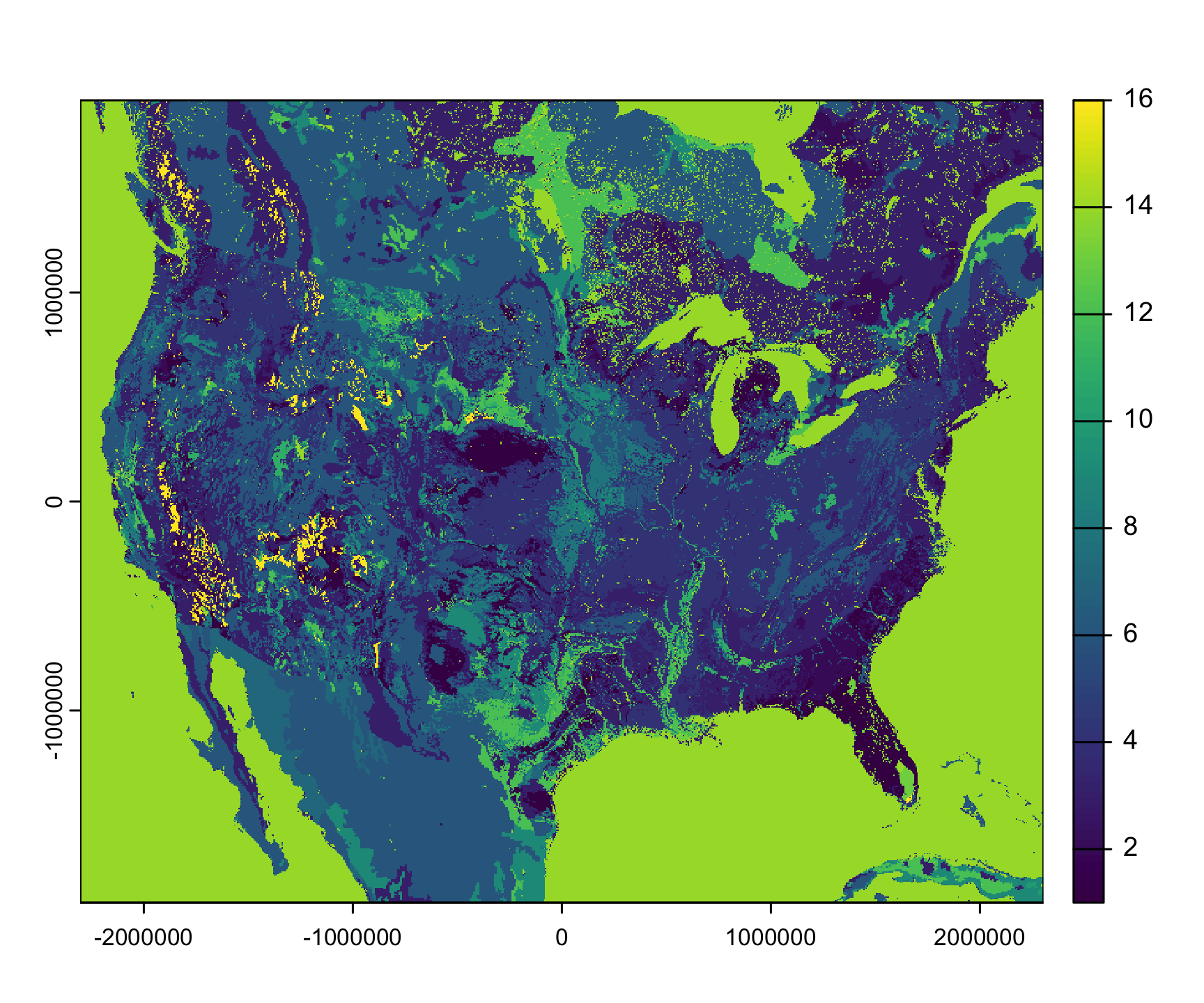
Return 2: GDAL

's3://spatial-water-noaa/nwm/CONUS/ISLTYP.tif' |> 
1  terra::rast() |>
  terra::plot()

1

Read tif data as raster with GDAL

Return 3: CSV

'https://raw.githubusercontent.com/nytimes/covid-19-data/master/us-counties.csv' |> 
1  readr::read_csv(n_max = 5)
# A tibble: 5 × 6
  date       county    state       fips cases deaths
  <date>     <chr>     <chr>      <dbl> <dbl>  <dbl>
1 2020-01-21 Snohomish Washington 53061     1      0
2 2020-01-22 Snohomish Washington 53061     1      0
3 2020-01-23 Snohomish Washington 53061     1      0
4 2020-01-24 Cook      Illinois   17031     1      0
5 2020-01-24 Snohomish Washington 53061     1      0

1

Read CSV data using csv reader

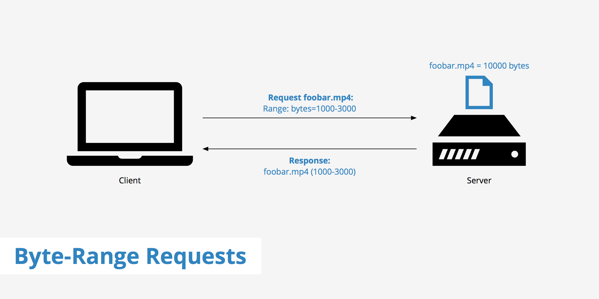
Note: Byte/HTTP Range Requests

• Byte range requests are a feature of HTTP. They allow clients to request only a portion of a resource

• Started with video buffering and bandwidth conservation

• Massively valuable in cloud compute

• Integral to cloud native geospatial

Objects in your Environment

Objects

• Objects store data (values) (my.school = “UCSB”)
• Objects can be changed according to our needs. (my.school = “CSU”)
• A object provides us with named storage that our programs can manipulate.
  1. Objects have a human readable name
  2. An operable value
  3. A location in memory where it is stored

So how do we define objects?

1. We can read them from a location (local or remote)

poudre.river <-  sf::read_sf('https://geoconnex.us/ref/mainstems/352913') 

poudre.river
Simple feature collection with 1 feature and 23 fields
Geometry type: LINESTRING
Dimension:     XY
Bounding box:  xmin: -105.8129 ymin: 40.41798 xmax: -104.6 ymax: 40.71387
Geodetic CRS:  WGS 84
# A tibble: 1 × 24
  id     head_nhdpv2_comid           head_nhdpv1_comid   fid outlet_nhdpv2_comid
  <chr>  <chr>                       <chr>             <int> <chr>              
1 352913 https://geoconnex.us/nhdpl… <NA>              18032 https://geoconnex.…
# ℹ 19 more variables: outlet_nhdpv1_comid <chr>, uri <chr>,
#   head_nhdpv2huc12 <chr>, head_2020huc12 <chr>, featuretype <chr>,
#   outlet_nhdpv2huc12 <chr>, outlet_2020huc12 <chr>,
#   downstream_mainstem_id <chr>, lengthkm <dbl>, superseded <lgl>,
#   encompassing_mainstem_basins <chr>, outlet_drainagearea_sqkm <dbl>,
#   new_mainstemid <chr>, name_at_outlet <chr>, head_rf1id <int>,
#   name_at_outlet_gnis_id <int>, outlet_rf1id <int>, datasets <chr>, …

2. We can define them in code!

Object Names & Values

• In both cases, the object name is arbitrary and helps reference values.

• Names are used by reader () of the program

• values are “bound” to a name using the = or <- assignment operators

a = 3
a <- 3

print(a)
[1] 3

• The result is the value 3 is bound to the name “a”.
• R can interpret the name as the object/value it holds.

# Allow computations
3*a
[1] 9

# Allow reassignment
a <- 5

# Allow operations
rep("TEXT", a)
[1] "TEXT" "TEXT" "TEXT" "TEXT" "TEXT"

Binding 101

It is easy to read this statement as “create an object, named x, containing the value 10”

x <- 10

• But this is a simplification!
• In actuality:
  • It’s creating a object of value 10
  • And binding that object to a name ‘x’
• Therefore the value (10) does not have a name, rather, the name (x) has a value (Subtle but important!!)

Object Address

• Objects have unique identifiers.
• These identifiers have a form that looks like the object’s memory “address”
• The actual memory addresses changes every time the code is run, so we use these identifiers instead.
• If you are interested in this, the Wikipedia page is great!

x <- 10

lobstr::obj_addr(x)
[1] "0x14c093cb8"

To illustate this…

In the code below, y doesn’t make another copy of the value 10, but instead creates an additional binding to the existing object.

x <- 10
y <- x

rlang::obj_address(x)
[1] "0x149ac8908"
rlang::obj_address(y)
[1] "0x149ac8908"

Equally, if we create two unique objects (even with the same value), they are different:

x2 <- 10
y2 <- 10

rlang::obj_address(x2)
[1] "0x1578e0000"
rlang::obj_address(y2)
[1] "0x1578df890"

This is because the values are buffered in memory rather then on hard disk!

Unchanging variables

Take this example as a final exploration:

x <- c(10, 10, 10)
y <- x

rlang::obj_address(x)
[1] "0x148d87f98"
rlang::obj_address(y)
[1] "0x148d87f98"

y[3] <- 6
y
[1] 10 10  6

rlang::obj_address(y)
[1] "0x13c3dadb8"

• While the value associated with y changed, the original object did not. Instead, R created a new object, a copy of of the original with one value changed, then rebound y to that object.

• This behaviour is called copy-on-modify. Understanding it will improve your understanding about the performance of R code.

• A related way to describe this behaviour is to say that R objects are unchangeable, or immutable.

• The more objects you make and modify, the more memeory is need to hold them!

• Which takes us to memory :)

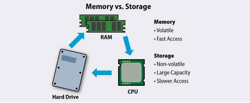
Computer Memory: Like a Dynamic Hard Disk

• Temporary Storage: Just like a hard disk stores data, computer memory (RAM) stores data, but it is temporary. It holds data and instructions that are actively used by the CPU.

• Dynamic: Unlike a static hard disk, memory is dynamic—it constantly updates as the system runs, reading and writing data quickly.

• Faster than Hard Disk: Memory operates at high speeds, enabling quicker access and retrieval of data compared to the relatively slower hard disk drives (HDDs).

• Volatility: Memory is volatile, meaning that once the computer is powered off, all stored data is lost. In contrast, hard disks retain data even when the system is powered down.

This is why memory (and clearing memory!) matters

So what can we do with objects?

• Remember our school example?

• We wanted to store information about the school as named values:

my.school <- "CSU"
lat <- 40.5715
lng <- -105.0752

• But these are very different kinds of information with defined capabilities.

• What would happen if we tried to add lng to lat?

lng + lat
[1] -64.5037

• What would happen if we tried to add lng to my.school?

lng + my.school
Error in lng + my.school: non-numeric argument to binary operator

• We see a non-numeric argument error telling us that name is not a numeric value. This is our first hint that values have different classes/types.

charToRaw(3)
Error in charToRaw(3): argument must be a character vector of length 1
charToRaw("3")
[1] 33

Why is the value “3” different the the value 3?

Computers (via R) convert bytes <-> hex <-> value

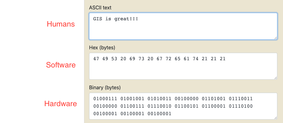
What’s the difference between 3 (the number) and ‘3’ (the character)?

• To a computer: nothing
• To us: meaning
• To software: hows its handled

Data Types

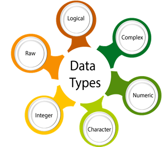
Data Types

Values in R can be one of 6 different types : 1. numeric (e.g. 2, 2.15) 2. integer (e.g. 2L) 3. character (e.g. "x", "Welcome!") 4. logical (e.g. TRUE, FALSE) 5. raw (e.g. holds bytes) 6. complex (e.g. 1+4i) - we are going to ignore

• The class function tells us what kind of object is it (high-level)
• The typeof function can tell us the object’s data type (low-level)

1. Numeric

• Values with decimals

• Of type “double” in computer science terms

• Default computational data type in R.

• Doubles can be specified in decimal (0.1234), scientific (1.23e4), or hexadecimal (0xcafe) form.

• There are three special values unique to doubles: Inf, -Inf, and NaN (not a number).

Numerics

(x = 4.75)

[1] 4.75

Numerics

(x = 4.75)
class(x)

[1] 4.75
[1] "numeric"

Numerics

(x = 4.75)
class(x)
typeof(x)

[1] 4.75
[1] "numeric"
[1] "double"

Numerics

(x = 4.75)
class(x)
typeof(x)

x * 2

[1] 4.75
[1] "numeric"
[1] "double"
[1] 9.5

Numerics

(x = 4.75)
class(x)
typeof(x)

x * 2
x + 2

[1] 4.75
[1] "numeric"
[1] "double"
[1] 9.5
[1] 6.75

Numerics

(x = 4.75)
class(x)
typeof(x)

x * 2
x + 2
x - 5

[1] 4.75
[1] "numeric"
[1] "double"
[1] 9.5
[1] 6.75
[1] -0.25

Numerics

(x = 4.75)
class(x)
typeof(x)

x * 2
x + 2
x - 5
x / 4

[1] 4.75
[1] "numeric"
[1] "double"
[1] 9.5
[1] 6.75
[1] -0.25
[1] 1.1875

Numerics

(x = 4.75)
class(x)
typeof(x)

x * 2
x + 2
x - 5
x / 4


x == 4

[1] 4.75
[1] "numeric"
[1] "double"
[1] 9.5
[1] 6.75
[1] -0.25
[1] 1.1875
[1] FALSE

2. Integer

• Values without decimals

• To create an integer in R you must follow the a number with an uppercase L.

• Take less memory then doubles but this is rarely an issue

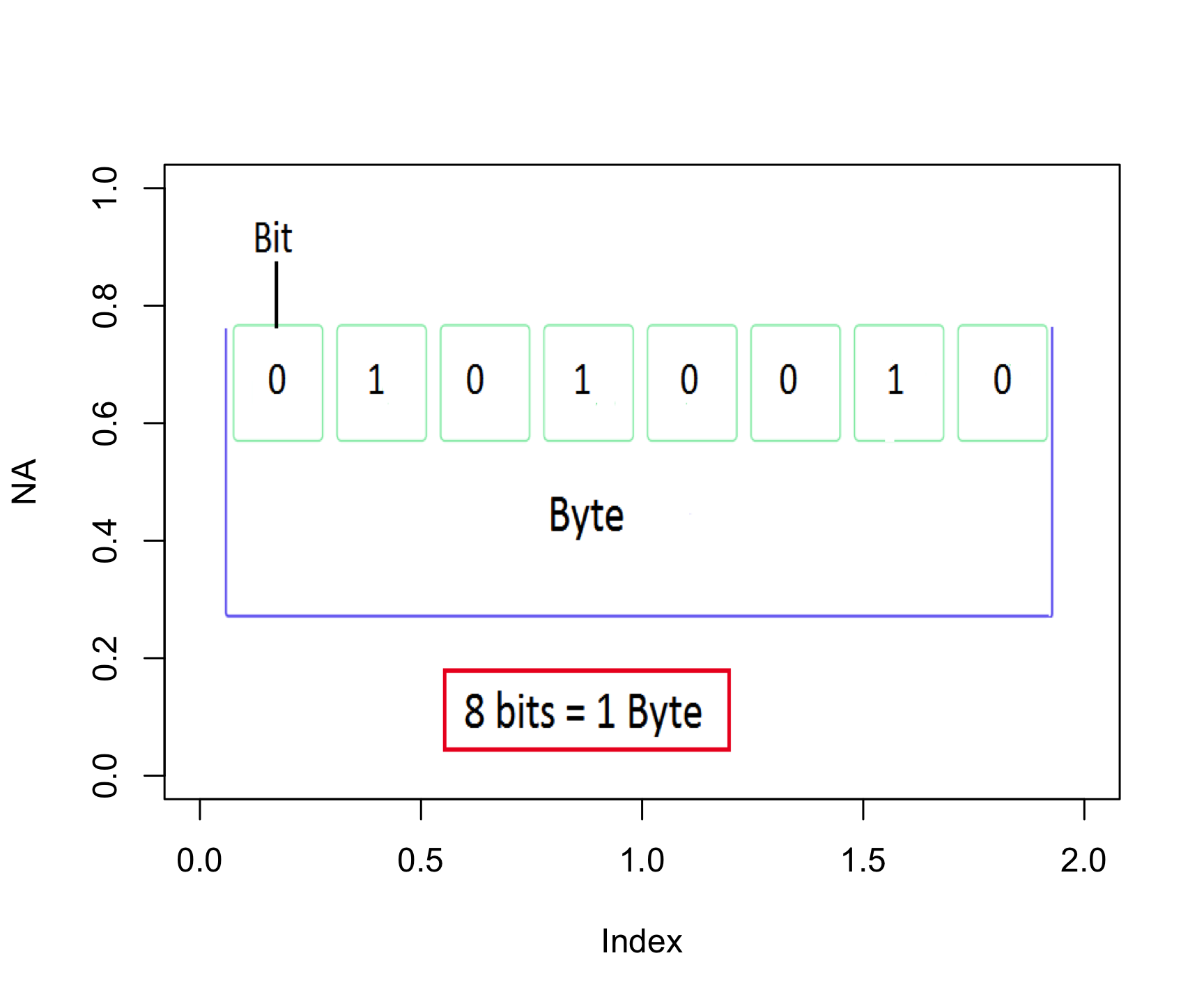
• One byte is 8 bits,

• Each bit can represent two values (0,1),

• One byte can hold 2⁸=256 values.

• used for (0 to 255) –or– (−128 to 127).

Integers

(x = 2)  # defaults to numeric

[1] 2

Integers

(x = 2)  # defaults to numeric
typeof(x)

[1] 2
[1] "double"

Integers

(x = 2)  # defaults to numeric
typeof(x)
(y = 2L)  # specifies integer

[1] 2
[1] "double"
[1] 2

Integers

(x = 2)  # defaults to numeric
typeof(x)
(y = 2L)  # specifies integer
typeof(y)

[1] 2
[1] "double"
[1] 2
[1] "integer"

Integers

(x = 2)  # defaults to numeric
typeof(x)
(y = 2L)  # specifies integer
typeof(y)
class(y)

[1] 2
[1] "double"
[1] 2
[1] "integer"
[1] "integer"

Integers

(x = 2)  # defaults to numeric
typeof(x)
(y = 2L)  # specifies integer
typeof(y)
class(y)

(t = 1L / 5L)

[1] 2
[1] "double"
[1] 2
[1] "integer"
[1] "integer"
[1] 0.2

Integers

(x = 2)  # defaults to numeric
typeof(x)
(y = 2L)  # specifies integer
typeof(y)
class(y)

(t = 1L / 5L)
typeof(t)

[1] 2
[1] "double"
[1] 2
[1] "integer"
[1] "integer"
[1] 0.2
[1] "double"

Integers

(x = 2)  # defaults to numeric
typeof(x)
(y = 2L)  # specifies integer
typeof(y)
class(y)

(t = 1L / 5L)
typeof(t)

## Casting

as.integer(c(4.1, 5.2, 6.3, 6.4))

[1] 2
[1] "double"
[1] 2
[1] "integer"
[1] "integer"
[1] 0.2
[1] "double"
[1] 4 5 6 6

3. Character

• character values stores text ranging in size from a single letter to a novel.

• surrounded by " (“here”) or ' (‘there’).

• Special characters are escaped with \; see ?Quotes for full details.

Characters

(x = "a")

[1] "a"

Characters

(x = "a")
(y = "bc")

[1] "a"
[1] "bc"

Characters

(x = "a")
(y = "bc")
(z = "GIS is Great!!!")

[1] "a"
[1] "bc"
[1] "GIS is Great!!!"

4. Logical

• Logical values store boolean values (TRUE and FALSE).

• Usefull for checking conditions and controlling the flow of a program.

• Or, for checking binary conditions (like on,off; open/closed; >100)

• The idea of the T/F boolean will be one of the most important in this class

• Logicals can be written in full (TRUE or FALSE), or abbreviated (T or F).

Logicals

u = TRUE

Logicals

u = TRUE
v = FALSE

Logicals

u = TRUE
v = FALSE
typeof(u)

[1] "logical"

Logicals

u = TRUE
v = FALSE
typeof(u)

# if u AND v are TRUE
u & v

[1] "logical"
[1] FALSE

Logicals

u = TRUE
v = FALSE
typeof(u)

# if u AND v are TRUE
u & v
# if u OR v are TRUE
u | v

[1] "logical"
[1] FALSE
[1] TRUE

Logicals

u = TRUE
v = FALSE
typeof(u)

# if u AND v are TRUE
u & v
# if u OR v are TRUE
u | v
# The opposite
!u

[1] "logical"
[1] FALSE
[1] TRUE
[1] FALSE

Logicals

u = TRUE
v = FALSE
typeof(u)

# if u AND v are TRUE
u & v
# if u OR v are TRUE
u | v
# The opposite
!u

# Equality / conditions
2 == 6

[1] "logical"
[1] FALSE
[1] TRUE
[1] FALSE
[1] FALSE

Logicals

u = TRUE
v = FALSE
typeof(u)

# if u AND v are TRUE
u & v
# if u OR v are TRUE
u | v
# The opposite
!u

# Equality / conditions
2 == 6
2 != 6

[1] "logical"
[1] FALSE
[1] TRUE
[1] FALSE
[1] FALSE
[1] TRUE

Logicals

u = TRUE
v = FALSE
typeof(u)

# if u AND v are TRUE
u & v
# if u OR v are TRUE
u | v
# The opposite
!u

# Equality / conditions
2 == 6
2 != 6

"test" == "test"

[1] "logical"
[1] FALSE
[1] TRUE
[1] FALSE
[1] FALSE
[1] TRUE
[1] TRUE

Logicals

u = TRUE
v = FALSE
typeof(u)

# if u AND v are TRUE
u & v
# if u OR v are TRUE
u | v
# The opposite
!u

# Equality / conditions
2 == 6
2 != 6

"test" == "test"

6 > 2

[1] "logical"
[1] FALSE
[1] TRUE
[1] FALSE
[1] FALSE
[1] TRUE
[1] TRUE
[1] TRUE

5. Raw

• The raw type is intended to hold raw bytes.
• Useful to introduce, but will only be used at a conceptual level.

Raws

(x <- charToRaw("GIS is great!"))

 [1] 47 49 53 20 69 73 20 67 72 65 61 74 21

Raws

(x <- charToRaw("GIS is great!"))
typeof(x)

 [1] 47 49 53 20 69 73 20 67 72 65 61 74 21
[1] "raw"

Raws

(x <- charToRaw("GIS is great!"))
typeof(x)

x[1]

 [1] 47 49 53 20 69 73 20 67 72 65 61 74 21
[1] "raw"
[1] 47

Raws

(x <- charToRaw("GIS is great!"))
typeof(x)

x[1]
rawToChar(x[1])

 [1] 47 49 53 20 69 73 20 67 72 65 61 74 21
[1] "raw"
[1] 47
[1] "G"

Raws

(x <- charToRaw("GIS is great!"))
typeof(x)

x[1]
rawToChar(x[1])
rawToHex(x[1])

 [1] 47 49 53 20 69 73 20 67 72 65 61 74 21
[1] "raw"
[1] 47
[1] "G"
[1] "47"

Raws

(x <- charToRaw("GIS is great!"))
typeof(x)

x[1]
rawToChar(x[1])
rawToHex(x[1])
rawToChar(x)

 [1] 47 49 53 20 69 73 20 67 72 65 61 74 21
[1] "raw"
[1] 47
[1] "G"
[1] "47"
[1] "GIS is great!"

Raws

(x <- charToRaw("GIS is great!"))
typeof(x)

x[1]
rawToChar(x[1])
rawToHex(x[1])
rawToChar(x)
rawToBits(x)

 [1] 47 49 53 20 69 73 20 67 72 65 61 74 21
[1] "raw"
[1] 47
[1] "G"
[1] "47"
[1] "GIS is great!"
  [1] 01 01 01 00 00 00 01 00 01 00 00 01 00 00 01 00 01 01 00 00 01 00 01 00 00
 [26] 00 00 00 00 01 00 00 01 00 00 01 00 01 01 00 01 01 00 00 01 01 01 00 00 00
 [51] 00 00 00 01 00 00 01 01 01 00 00 01 01 00 00 01 00 00 01 01 01 00 01 00 01
 [76] 00 00 01 01 00 01 00 00 00 00 01 01 00 00 00 01 00 01 01 01 00 01 00 00 00
[101] 00 01 00 00

Raws

(x <- charToRaw("GIS is great!"))
typeof(x)

x[1]
rawToChar(x[1])
rawToHex(x[1])
rawToChar(x)
rawToBits(x)

raw

 [1] 47 49 53 20 69 73 20 67 72 65 61 74 21
[1] "raw"
[1] 47
[1] "G"
[1] "47"
[1] "GIS is great!"
  [1] 01 01 01 00 00 00 01 00 01 00 00 01 00 00 01 00 01 01 00 00 01 00 01 00 00
 [26] 00 00 00 00 01 00 00 01 00 00 01 00 01 01 00 01 01 00 00 01 01 01 00 00 00
 [51] 00 00 00 01 00 00 01 01 01 00 00 01 01 00 00 01 00 00 01 01 01 00 01 00 01
 [76] 00 00 01 01 00 01 00 00 00 00 01 01 00 00 00 01 00 01 01 01 00 01 00 00 00
[101] 00 01 00 00
function (length = 0L) 
.Internal(vector("raw", length))
<bytecode: 0x13f4ec8e8>
<environment: namespace:base>

Bonus: Time

Representing time is a somewhat complex problem. There are different calendars, hours, days, months, and leap years to consider. As a basic introduction, here is simple way to create date values.

Times

(start <- as.Date('2020-08-03'))

[1] "2020-08-03"

Times

(start <- as.Date('2020-08-03'))
(end   <- as.Date('2020-09-11'))

[1] "2020-08-03"
[1] "2020-09-11"

Times

(start <- as.Date('2020-08-03'))
(end   <- as.Date('2020-09-11'))
typeof(start)

[1] "2020-08-03"
[1] "2020-09-11"
[1] "double"

Times

(start <- as.Date('2020-08-03'))
(end   <- as.Date('2020-09-11'))
typeof(start)

end - start

[1] "2020-08-03"
[1] "2020-09-11"
[1] "double"
Time difference of 39 days

Times

(start <- as.Date('2020-08-03'))
(end   <- as.Date('2020-09-11'))
typeof(start)

end - start

format(start, "%m")

[1] "2020-08-03"
[1] "2020-09-11"
[1] "double"
Time difference of 39 days
[1] "08"

Times

(start <- as.Date('2020-08-03'))
(end   <- as.Date('2020-09-11'))
typeof(start)

end - start

format(start, "%m")
format(start, "%y")

[1] "2020-08-03"
[1] "2020-09-11"
[1] "double"
Time difference of 39 days
[1] "08"
[1] "20"

Times

(start <- as.Date('2020-08-03'))
(end   <- as.Date('2020-09-11'))
typeof(start)

end - start

format(start, "%m")
format(start, "%y")
format(start, "%Y")

[1] "2020-08-03"
[1] "2020-09-11"
[1] "double"
Time difference of 39 days
[1] "08"
[1] "20"
[1] "2020"

And there are more advanced classes as well that capture date and time. We will get into these latter in class.

as.POSIXlt(start)
[1] "2020-08-03 UTC"
as.POSIXct(start)
[1] "2020-08-03 UTC"

Summary

Workflows

R Project

• An R project is a working directory designated with a .RProj file.

.
└── github
└── my_project
└── my_project.Rproj
└── .gitignore

• When you open a project:
  • In RStudio: File –> Open Project
• Outside RStudio: double–clicking on the .Rproj file

the working directory is automatically be set to the directory where .RProj file is located!

• Allows you to work with relative rather then absolute paths!

• Consider creating a new R Project whenever you are starting a new project.

• This will enforce a self contained project with associated data, scripts, and output

Building the rest of the Project…

README.md

README files are the “users manual” for the project

• What is the name
• purpose
• installation directions
• rules of use

We use the md extension (markdown) because GitHub autorenders pure Markdown

For us, a title, 1-2 sentence description and data attribution is plenty.

touch README.md

.
└── github
└── my_project
└── my_project.Rproj
└── .gitignore
└── README.md

R or (src)

• A directory call R (or src) is used to hold all scripts used in the analysis.
• The can be data processing, analysis, or figure generation sripcts

mkdir R # make a R directory
cd R # Enter the R directory
touch some-code.R # make a file
touch utils.R # make a file
cd.. # move back up to my_project directory

.
├── github
├── my_project
├── my_project.Rproj
├── .gitignore
├── README.md
└── R
    └── some-code.R
    └── utils.R

imgs (or img or figs or output)

This folder is for things that are saved as a result of your scripts - Plot images - Maps - Ect

mkdir imgs # make a imgs directory

.
├── github
├── my_project
├── my_project.Rproj
├── .gitignore
├── README.md
├── R
│   └── some-code.R
|   └── utils.R
└── img
     └── cool-img.png

docs (only docs)

• the docs folder should hold your Qmd files and there rendered output
• Github Pages can be deployed from the docs folder making this a good practice if you want to share information over the web in a free secure way

mkdir docs # make a docs directory
cd docs # Enter the docs directory
touch index.Qmd # make a file
cd .. # move back up to my_project directory

.
├── github
├── my_project
├── my_project.Rproj
├── .gitignore
├── README.md
├── R
│   └── some-code.R
|   └── utils.R
├── img
|   └── cool-img.png
├── docs
├── index.Rmd
└── index.html

data

• the data folder is an storage archive for raw data

• It’s crucial to make a distinction between source/raw data and generated data:

  Treat source/raw data as read-only Treat generated data as disposable.

• Some might separate raw and generated data into separate sub directories. I prefer to segment them through the naming

mkdir data # make a data directory

.
├── github
├── my_project
├── my_project.Rproj
├── .gitignore
├── README.md
├── R
│   └── some-code.R
|   └── utils.R
├── img
|   └── some-code.R
├── docs
|   └── index.Rmd
|   └── index.html
└── data
    └── data.csv

Rules…

1. Treat data as read only
2. Treat generated output as disposable
3. Other then that, structure should match the project goals and is flexable!

The goal for workflows:

Tip

We will do everything in well-annotated, organized scripts that contain streamlined and easy-to-follow records of our entire analyses from raw data through final reports, with unbreakable file paths and with a complete history of changes made.

• Well-annotated: Through documentation and comments

• Organized: Directory Strucutre

• Raw Data: Keep raw data raw!

• Final Reports: Rmarkdown files

• Unbreakable Paths: .Rproj to the rescue

• Complete History: Version control with git and GitHub

Next Time:

Daily Assignment: Your First Project

Next Topic: Your Tools: Interactive Walk Though

Artwork by @allison_horst