Week 3
Writing Functions
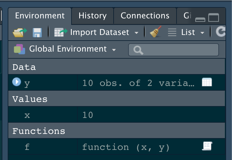
Our own functions are visable as objects in the environemnt
Using our function:
Like any object, we have to run the lines of code to save it as an object before we can use it directly in our code:
But then …
Cities
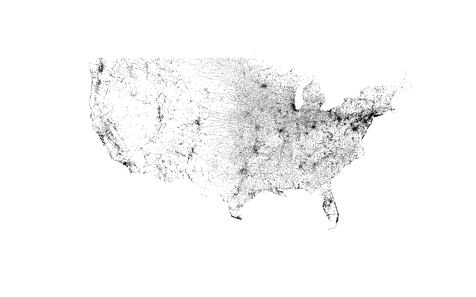
Point-in-Polygon Case Study
The power of GIS lies in analyzing multiple data sources together.
Often the answer you want lies in many different layers and you need to do some analysis to extract and compile information.
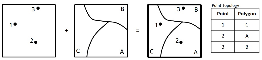
One common analysis is Points-in-Polygon (PIP).
PIP is useful when you want to know how many - or what kind of - points fall within the bounds of each polygon
Data
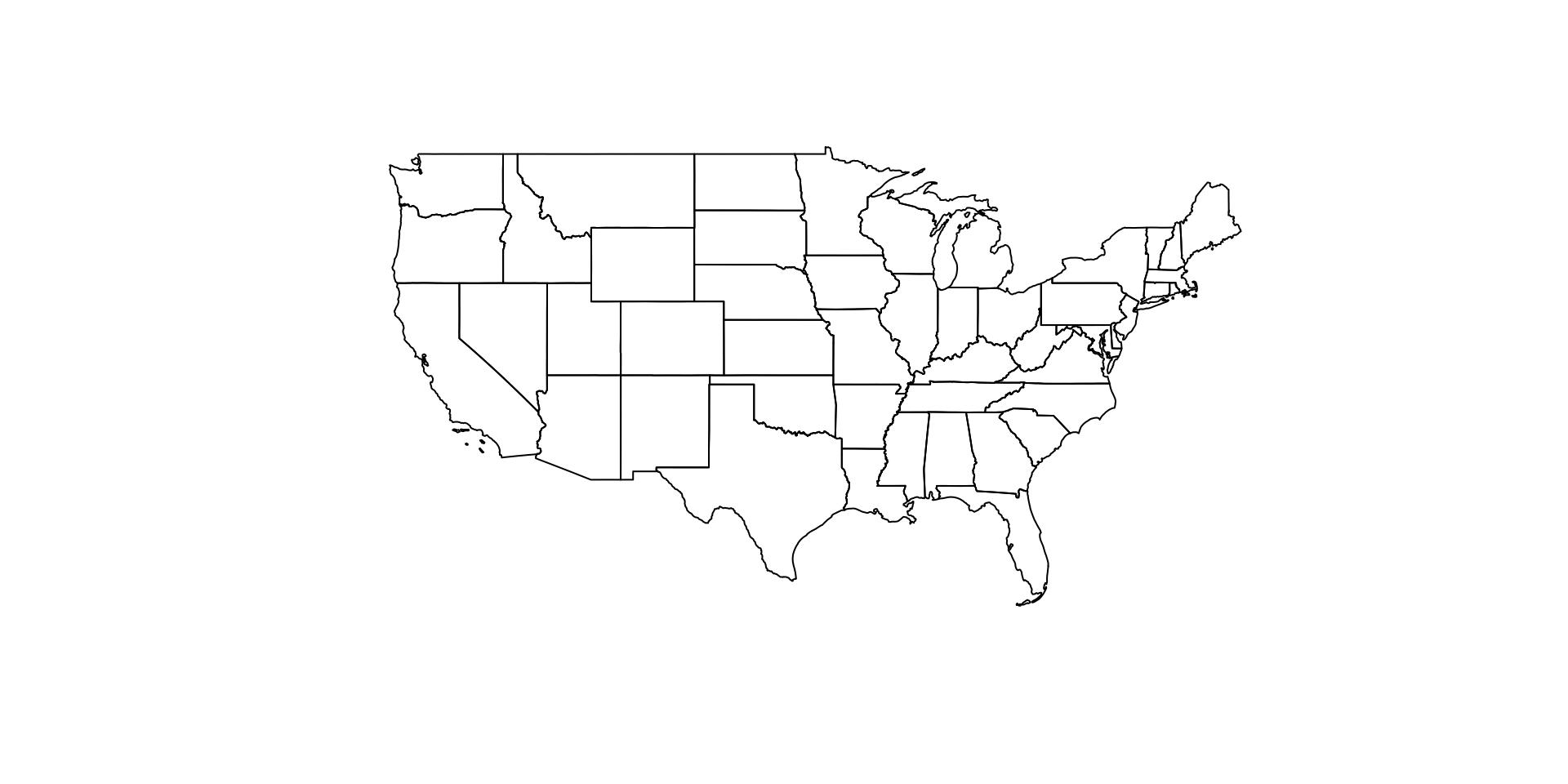
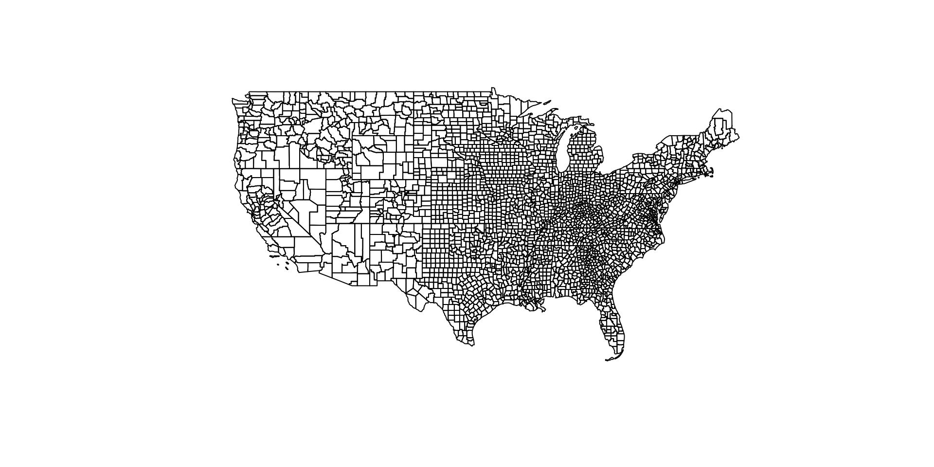
CONUS counties
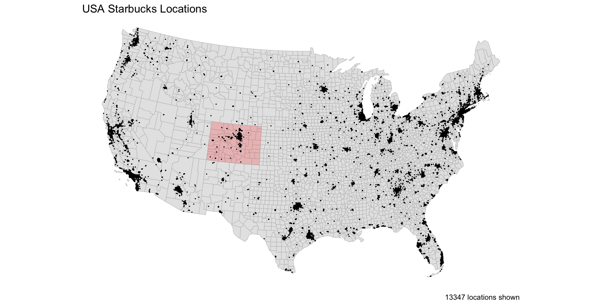
CONUS Starbucks
Colorado Counties
Step 3: Combine the processes …

Test

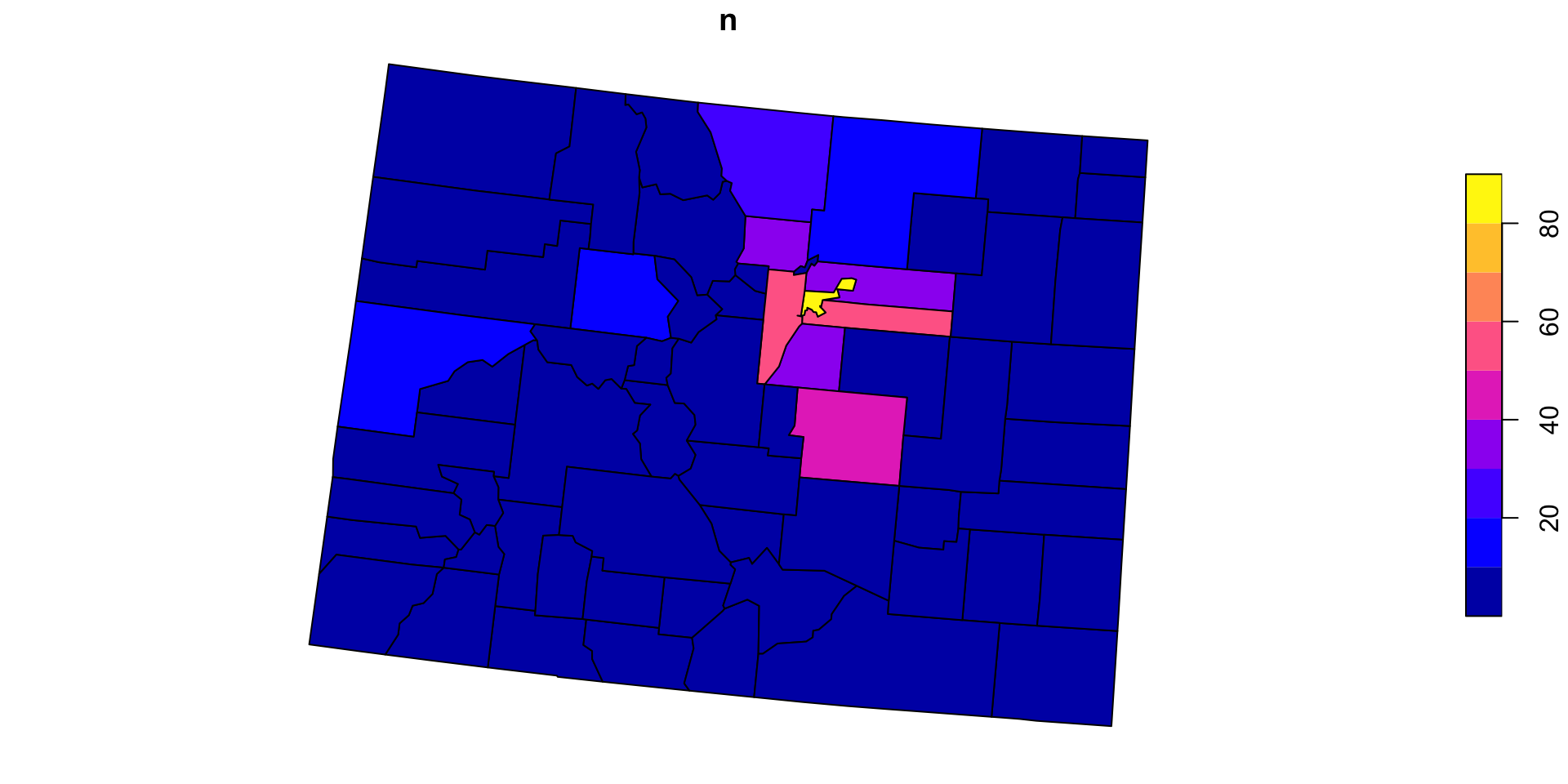
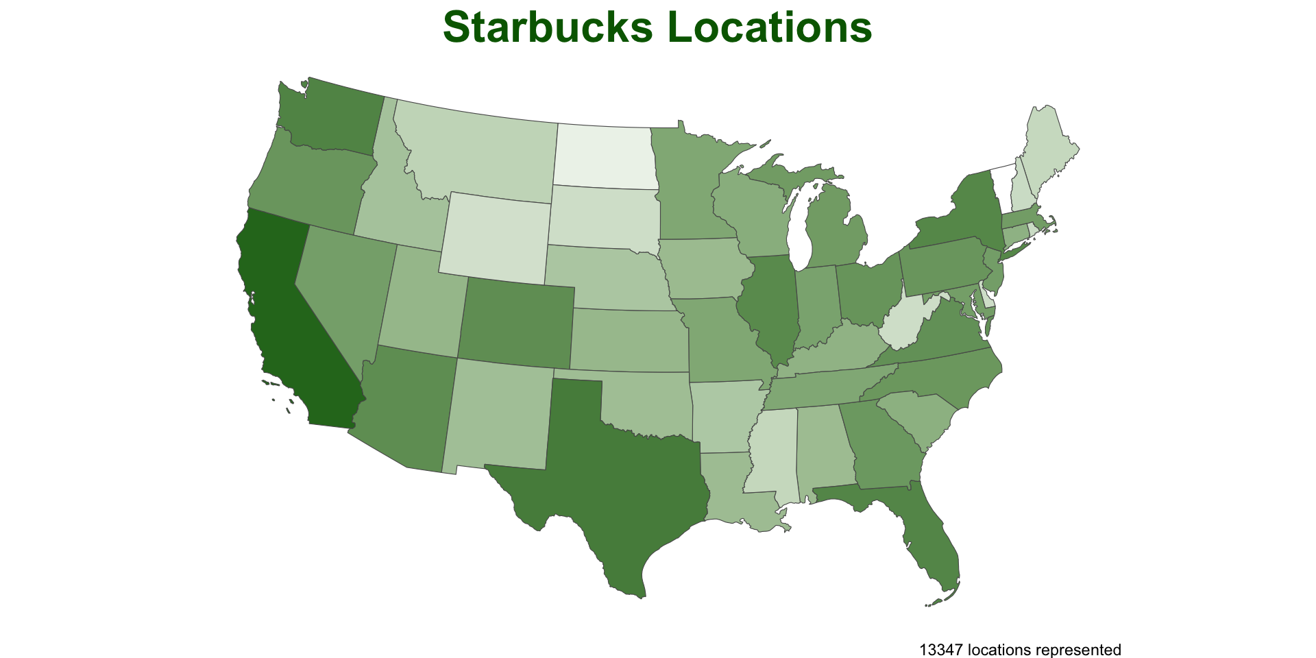
Applying the new function
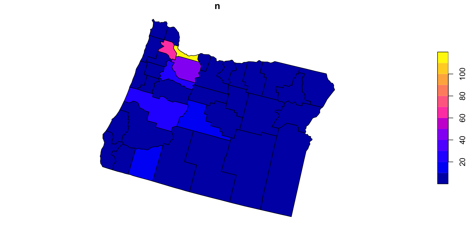
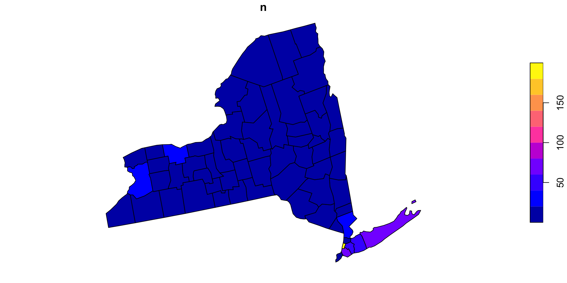
- Here, we can apply the PIP function over states and count by
name
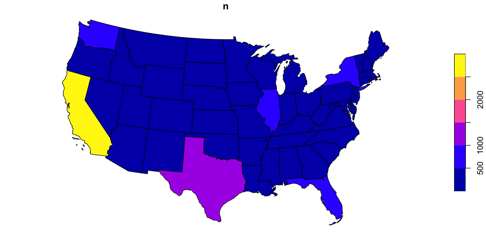
Test
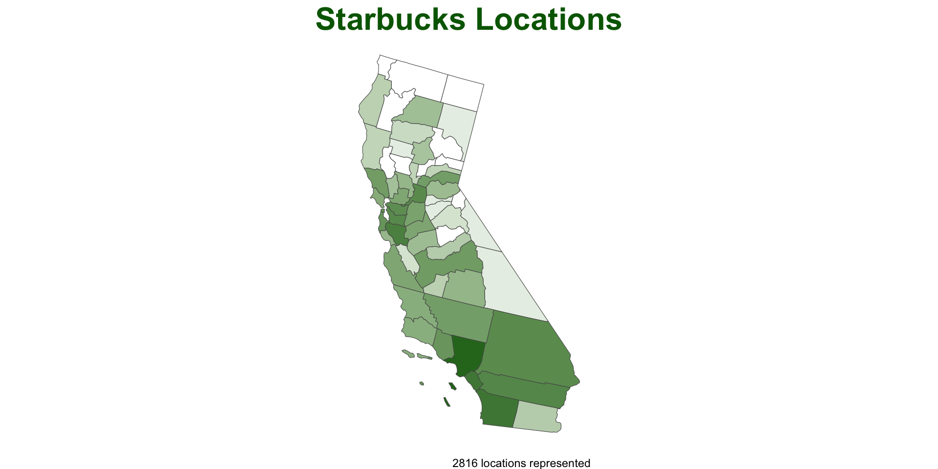
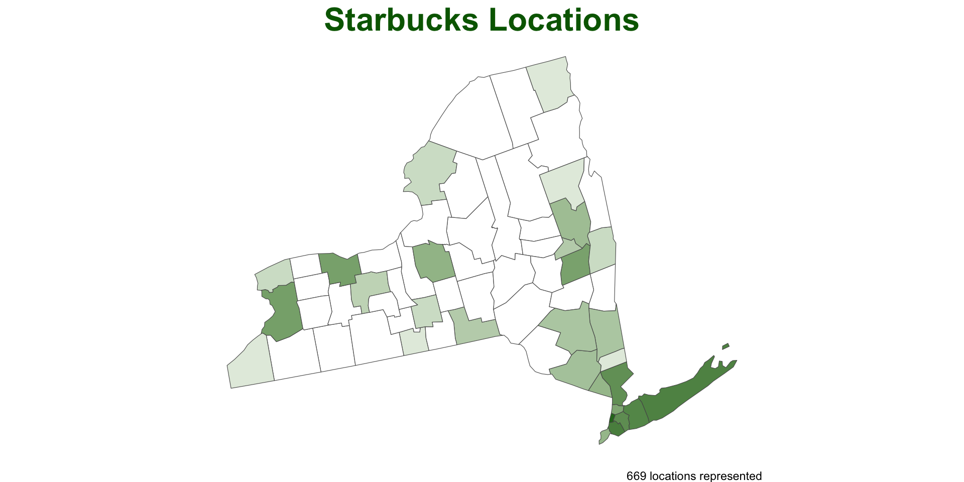
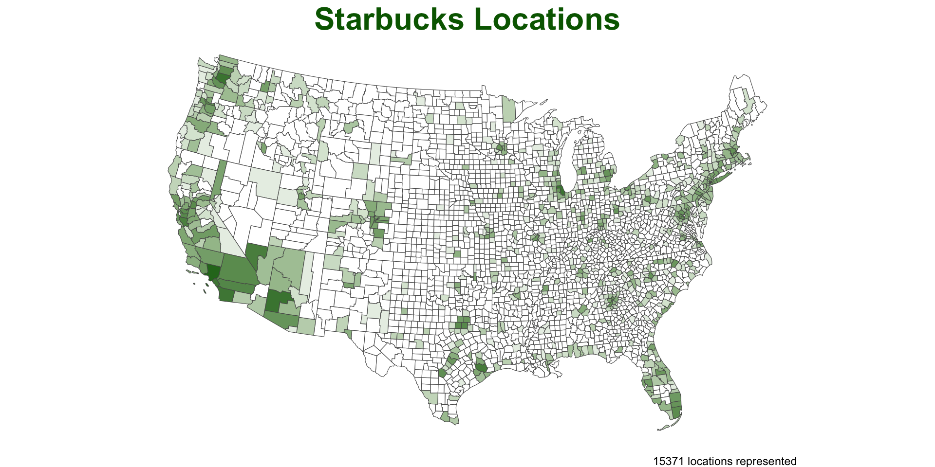
PIP –> Plotting Method
We can use our functions right out of the box for this data
But… somethings are not quite right..
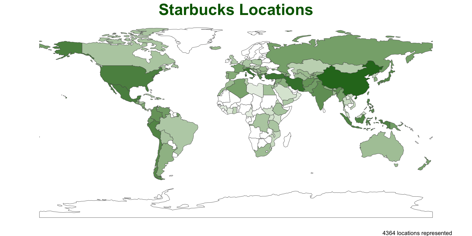
Modify for our analysis …
Improve the anaylsis…
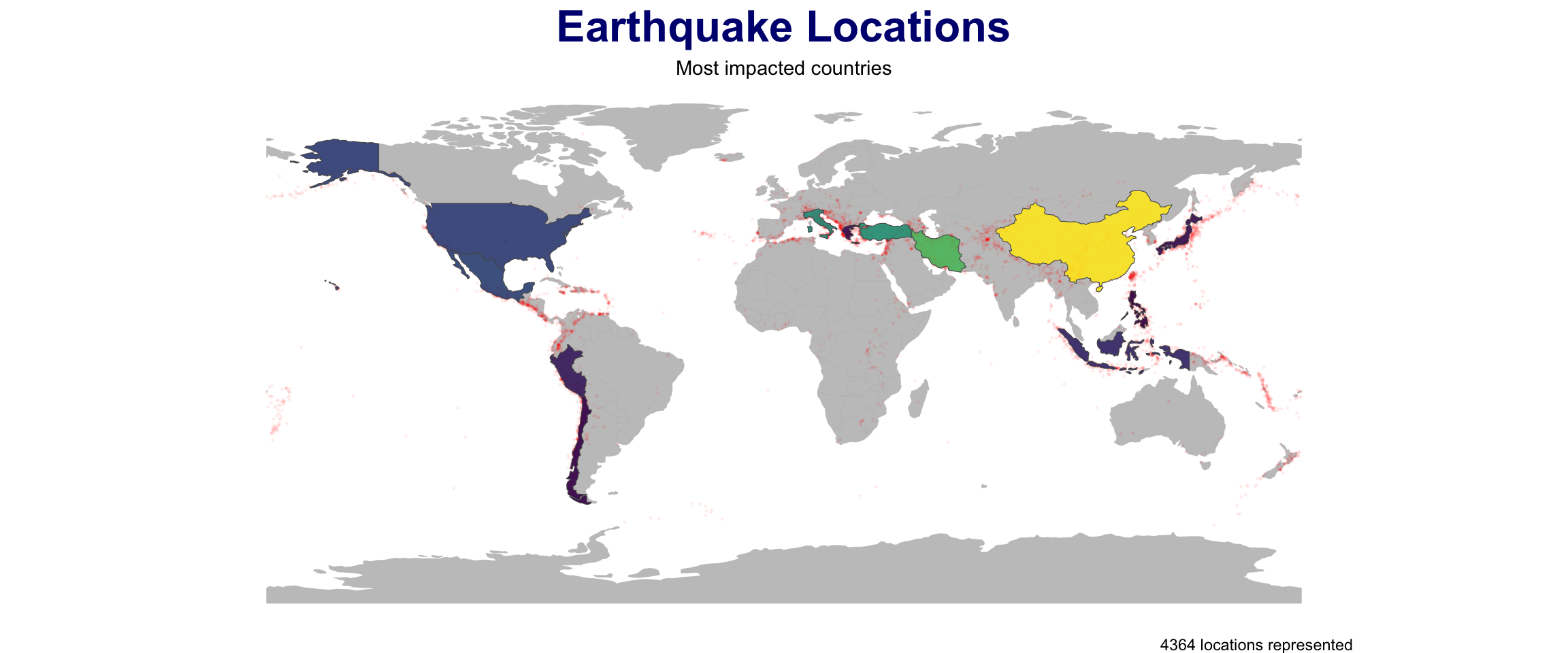
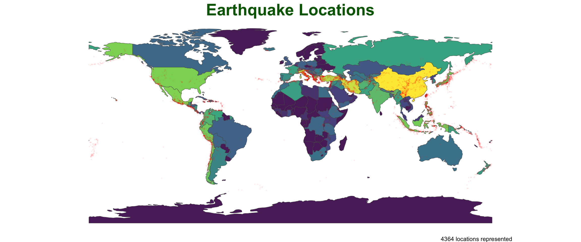
point_in_polygon3(quakes, countries, var = "ADMIN") |>
plot_pip() +
labs(title = "Earthquake Locations",
subtitle = "Most impacted countries") +
theme(plot.subtitle = element_text(hjust = .5),
plot.title = element_text(color = "navy")) +
scale_fill_viridis_c() +
geom_sf(data = quakes, size = .3, alpha = .05, col = 'red') +
gghighlight::gghighlight(n > (mean(n) + sd(n)))