Interactive Mapping in R

Leaflet

This is the supplementary notes and examples for an introduction to leaflet.

It is based on data and examples seen in class

Built on the excellent tutorial from RStudio

---

If not already installed, install leaflet:

install.packages("leaflet")

Then attach the library:

library(leaflet)

Bring in the other needed libraries:

library(sf)
library(tidyverse)
library(USAboundaries)

---

Basic Usage

Creating a Leaflet map requires a few basic steps (not dissimilar to ggplot):

1. Initialize a map widget by calling leaflet().

2. Add layers (i.e., features) to the map by using layer functions (e.g. addTiles, addMarkers, addPolygons,…)

3. Print the map widget to display it.

---

Here’s a basic example:

leaflet() |>
  addTiles() |>
  addMarkers(lng=-105.0848, lat=40.5729, popup="CSU")

---

• By default, leaflet sets the view of the map to the range of latitude/longitude data in the map layers

• You can adjust these if needed using:

  • setView(): sets the center of the map view and the zoom level;

  • fitBounds(): fits the view into the rectangle [lng1, lat1] – [lng2, lat2];

  • clearBounds() clears the bound

---

Basemaps

Default (OpenStreetMap) Tiles

The easiest way to add tiles is by calling addTiles() with no arguments; by default, OpenStreetMap tiles are used.

leaflet() |> 
  setView(lng=-105.0848, lat=40.5729, zoom = 16) |> 
  addTiles()

Third-Party Tiles

• Many third-party basemaps can be added using the addProviderTiles() function

• As a convenience, leaflet provides a named list of all the third-party tile providers supported by the plugin: just type providers$ and choose from one of the options.

length(providers)

#> [1] 233

names(providers) |> 
  head()

#> [1] "OpenStreetMap"        "OpenStreetMap.Mapnik" "OpenStreetMap.DE"    
#> [4] "OpenStreetMap.CH"     "OpenStreetMap.France" "OpenStreetMap.HOT"

Note that some tile set providers require you to register. You can pass access tokens/keys, and other options, to the tile provider by populating the options argument with the providerTileOptions() function.

• I would personal stick with the OSM, CartoDB, ESRI, and Stamen servers … [see more here] (https://leaflet-extras.github.io/leaflet-providers/preview/)

Below are a few examples:

CartoDB

leaflet() |> 
  setView(lng=-105.0848, lat=40.5729, zoom = 16) |> 
  addProviderTiles(providers$CartoDB)

ESRI Imagery

leaflet() |> 
  setView(lng=-105.0848, lat=40.5729, zoom = 16) |> 
  addProviderTiles(providers$Esri.WorldImagery)

Combining Tile Layers

You can stack multiple tile layers if the front tiles have some level of opacity. Here we layer the Stamen.TonerLines with aerial imagery

leaflet() |> 
  setView(lng=-105.0848, lat=40.5729, zoom = 14) |> 
  addProviderTiles(providers$Esri.WorldImagery) |> 
  addProviderTiles(providers$Stadia.StamenTonerLines,
                   options = providerTileOptions(opacity = .5)) 

---

Markers

Markers are one way to identify point information on a map:

---

Example Starbucks data:

(starbucks = read_csv('data/directory.csv') |> 
  filter(City %in% c("Fort Collins", "Loveland"),
         `State/Province` == "CO") |> 
  st_as_sf(coords = c("Longitude", "Latitude"), crs = 4326) |> 
  select(store_name = `Store Name`, phone = `Phone Number`, address = `Street Address`, city = City, brand = Brand))

#> Simple feature collection with 21 features and 5 fields
#> Geometry type: POINT
#> Dimension:     XY
#> Bounding box:  xmin: -105.12 ymin: 40.38 xmax: -105.01 ymax: 40.61
#> Geodetic CRS:  WGS 84
#> # A tibble: 21 × 6
#>    store_name                phone address city  brand        geometry
#>    <chr>                     <chr> <chr>   <chr> <chr>     <POINT [°]>
#>  1 Harmony & Timberline-For… 970-… 4609 S… Fort… Star… (-105.04 40.52)
#>  2 Safeway-Fort Collins #10… 970-… 460A S… Fort… Star… (-105.08 40.58)
#>  3 Scotch Pines              970-… 2601 S… Fort… Star… (-105.06 40.55)
#>  4 King Soopers-Fort Collin… 970-… 2602 S… Fort… Star… (-105.04 40.55)
#>  5 Safeway-Fort Collins #29… 970-… 2160 W… Fort… Star… (-105.12 40.55)
#>  6 Harmony & JFK             (970… 250 E.… Fort… Star… (-105.07 40.52)
#>  7 Safeway-Fort Collins #15… 970-… 1426 E… Fort… Star… (-105.05 40.52)
#>  8 SuperTarget Fort Collins… <NA>  2936 C… Fort… Star… (-105.08 40.53)
#>  9 King Soopers-Fort Collin… 970-… 1015 S… Fort… Star… (-105.12 40.57)
#> 10 King Soopers-Ft. Collins… 970-… 1842 N… Fort… Star… (-105.08 40.61)
#> # ℹ 11 more rows

Markers

Markers are added using the addMarkers or addAwesomeMarkers

Their default appearance is a blue dropped pin.

As with most layer functions, - the popup argument adds a message to be displayed on click - the label argument display a text label either on hover

leaflet() |> 
  addProviderTiles(providers$CartoDB) |> 
  addMarkers(data = starbucks, popup = ~store_name, label = ~city)

Awesome Icons

Using the Font Awesome Icons seen in lab one, we can make markers with more specific coloring and icons

• Here we define the icon as a green marker with a coffee icon from the fa library
• For fun we can make the coffee cups spin…

We then use addAwesomeMarkers to spcifiy the icon we created using the icon argument:

icons = awesomeIcons(icon = 'coffee', markerColor = "green", library = 'fa', spin = TRUE)

leaflet(data = starbucks) |> 
  addProviderTiles(providers$CartoDB) |> 
  addAwesomeMarkers(icon = icons, popup = ~store_name)

Custom Popups

You can use HTML, CSS, and Java Script to modify your pop-ups

For example, we can associate the name of the Starbucks locations with their google maps URL as an hyper reference (href):

starbucks = starbucks |> 
  mutate(url = paste0('https://www.google.com/maps/place/',
                      gsub(" ", "+", address), "+",
                      gsub(" ", "+", city)))

pop = paste0('<a href=', starbucks$url, '>', starbucks$store_name, "</a>")
head(pop)

#> [1] "<a href=https://www.google.com/maps/place/4609+S+Timberline+Rd,+Unit+A101+Fort+Collins>Harmony & Timberline-Fort Collins</a>"
#> [2] "<a href=https://www.google.com/maps/place/460A+South+College+Fort+Collins>Safeway-Fort Collins #1071</a>"                    
#> [3] "<a href=https://www.google.com/maps/place/2601+S+Lemay,+Ste+130+Fort+Collins>Scotch Pines</a>"                               
#> [4] "<a href=https://www.google.com/maps/place/2602+S+Timberline+Rd+Fort+Collins>King Soopers-Fort Collins #97</a>"               
#> [5] "<a href=https://www.google.com/maps/place/2160+W+Drake+Rd,+Unit+6+Fort+Collins>Safeway-Fort Collins #2913</a>"               
#> [6] "<a href=https://www.google.com/maps/place/250+E.+Harmony+Road+Fort+Collins>Harmony & JFK</a>"

We can then add our custom popup to our icons:

leaflet(data = starbucks) |>
  addProviderTiles(providers$CartoDB) |> 
  addAwesomeMarkers(icon = icons, 
                    label = ~address, popup = pop)

Circle Markers

Circle markers are much like regular circles (shapes), except their radius in onscreen pixels stays constant regardless of zoom level (z).

leaflet(data = starbucks) |>
  addProviderTiles(providers$CartoDB) |> 
  addCircleMarkers(label = ~address, popup = pop)

Marker Clustering

Sometimes while mapping many points, it is useful to cluster them. For example lets plot all starbucks in the world!

all_co = read_csv('data/directory.csv') |> 
  filter(!is.na(Latitude)) |> 
  st_as_sf(coords = c("Longitude", "Latitude"), crs = 4326) 

leaflet(data = all_co) |> 
  addProviderTiles(providers$CartoDB) |> 
  addMarkers(clusterOptions = markerClusterOptions())

---

Adding color ramps

• Colors can be add by factor, numeric, bins, or quartiles using the built in leaflet functions
• Each of these are defined by a palette, and a domain

The palette argument can be any of the following:

• A character vector of RGB or named colors.
  • Examples: palette(), c(“#000000”, “#0000FF”, “#FFFFFF”), topo.colors(10)
• The name of an RColorBrewer palette
  • Examples: “BuPu” or “Greens”.
• The full name of a viridis palette:
  • Examples: “viridis”, “magma”, “inferno”, or “plasma”.
• A function that receives a single value between 0 and 1 and returns a color.
  • Examples: colorRamp(c(“#000000”, “#FFFFFF”), interpolate = “spline”).

The domain is the values - named by variable - that the color palette should range over

# ?colorFactor

# Create a palette that maps factor levels to colors
pal <- colorFactor(c("darkgreen", "navy"), domain = c("Goleta", "Santa Barbara"))

leaflet(data = starbucks) |> addProviderTiles(providers$CartoDB) |> 
  addCircleMarkers(color = ~pal(city), fillOpacity = .5, stroke = FALSE)

---

Shapes (Polylines, Polygons, Circles)

Getting some data …

(covid = readr::read_csv('https://raw.githubusercontent.com/nytimes/covid-19-data/master/live/us-states.csv') |> 
  filter(date == max(date)) |> 
  right_join(USAboundaries::us_states(), by = c("state" = "name")) |> 
  filter(!stusps %in% c("AK","PR", "HI")) |> 
  st_as_sf())

#> Simple feature collection with 49 features and 16 fields
#> Geometry type: MULTIPOLYGON
#> Dimension:     XY
#> Bounding box:  xmin: -124.7258 ymin: 24.49813 xmax: -66.9499 ymax: 49.38436
#> Geodetic CRS:  WGS 84
#> # A tibble: 49 × 17
#>    date       state    fips   cases deaths statefp statens affgeoid geoid stusps
#>    <date>     <chr>    <chr>  <dbl>  <dbl> <chr>   <chr>   <chr>    <chr> <chr> 
#>  1 2023-03-24 Tenness… 47    2.46e6  29035 47      013258… 0400000… 47    TN    
#>  2 2023-03-24 Michigan 26    3.07e6  42311 26      017797… 0400000… 26    MI    
#>  3 2023-03-24 Massach… 25    2.23e6  24441 25      006069… 0400000… 25    MA    
#>  4 2023-03-24 Maryland 24    1.37e6  16672 24      017149… 0400000… 24    MD    
#>  5 2023-03-24 Iowa     19    9.07e5  10770 19      017797… 0400000… 19    IA    
#>  6 2023-03-24 Maine    23    3.20e5   2981 23      017797… 0400000… 23    ME    
#>  7 2023-03-24 Texas    48    8.45e6  94518 48      017798… 0400000… 48    TX    
#>  8 2023-03-24 Louisia… 22    1.58e6  18835 22      016295… 0400000… 22    LA    
#>  9 2023-03-24 Kansas   20    9.41e5  10232 20      004818… 0400000… 20    KS    
#> 10 2023-03-24 Kentucky 21    1.72e6  18348 21      017797… 0400000… 21    KY    
#> # ℹ 39 more rows
#> # ℹ 7 more variables: lsad <chr>, aland <dbl>, awater <dbl>, state_name <chr>,
#> #   state_abbr <chr>, jurisdiction_type <chr>, geometry <MULTIPOLYGON [°]>

Polygons

Adding those cases counts to polygons over a YlOrRd color ramp

leaflet() |> 
  addProviderTiles(providers$CartoDB) |> 
  addPolygons(data = covid, 
              fillColor  = ~colorQuantile("YlOrRd", cases)(cases),
              color = NA,
              label = ~state_name)

Circles

leaflet() |> 
  addProviderTiles(providers$CartoDB.DarkMatter) |> 
  addCircles(data = st_centroid(covid), 
             fillColor  = ~colorQuantile("YlOrRd", cases)(cases),
             color = NA,
             fillOpacity = .5,
             radius = ~cases/50,
             label = ~state)

Web based data

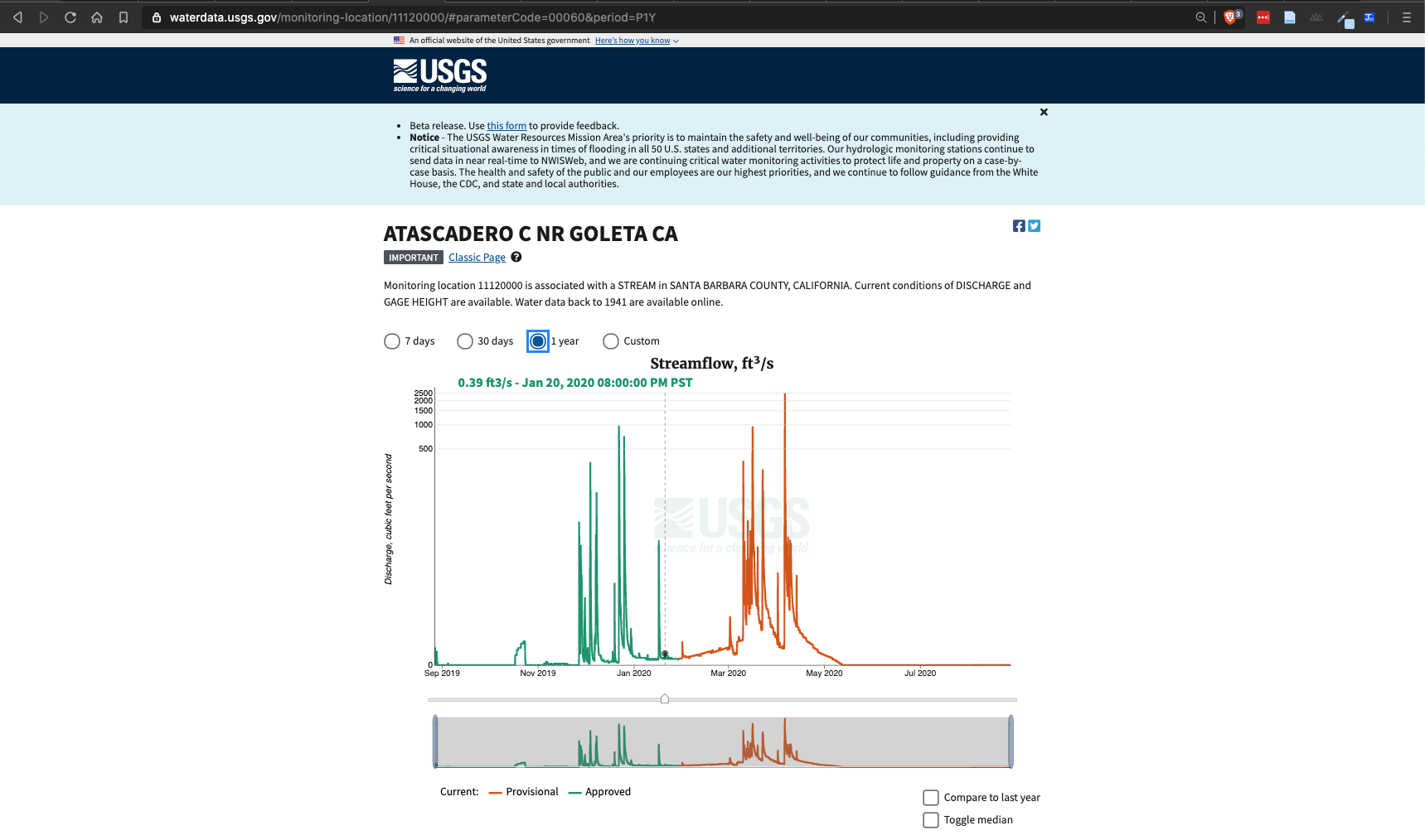
USGS Gage near UCSB: ID-11120000

https://waterdata.usgs.gov/monitoring-location/11120000/

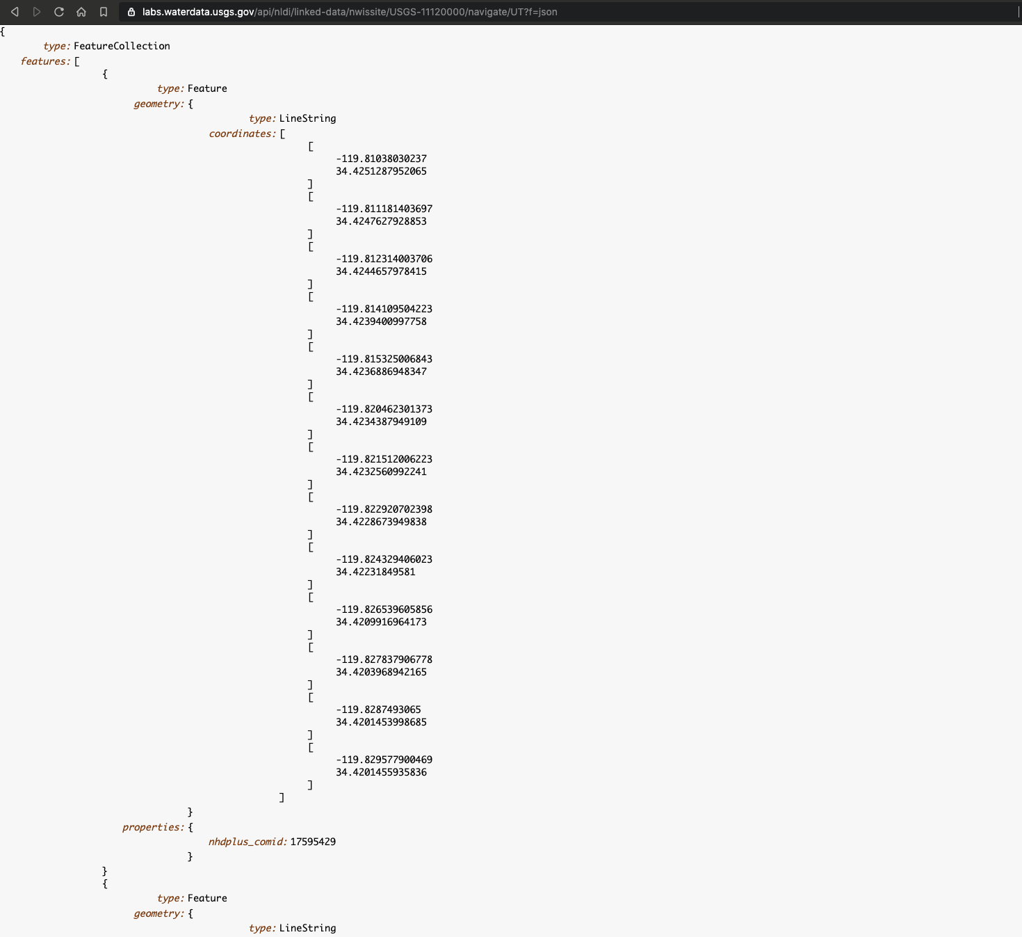
Network Linked Data (GeoJSON)

https://labs.waterdata.usgs.gov/api/nldi/linked-data/nwissite/USGS-11120000/navigate/UT

Trance the Upper Tributary (UT) of the USGS-11120000

Adding “Web data” to the map

id = "11120000"

# base URL
(base = dataRetrieval:::pkg.env$nldi_base)

#> [1] "https://api.water.usgs.gov/nldi/linked-data/"

# Reading sf for URLs in line
leaflet() |> 
  addProviderTiles(providers$CartoDB) |> 
  addPolylines(data = read_sf(paste0(base,'nwissite/USGS-',id,'/navigate/UT'))) |> 
  addPolygons(data =  read_sf(paste0(base,'nwissite/USGS-',id,'/basin')), 
              fillColor =  "transparent", color = "black")

---

WMS Tiles

WMS tiles can be added directly to a map. Here we use the NEXRAD rainfall information (refelctivity) from the Iowa Mesonet Program

(You may need to scroll out to find an)

conus = filter(us_states(), !stusps %in% c("AK", "PR", "HI"))

leaflet() |> 
  addProviderTiles(providers$CartoDB) |> 
  addPolygons(data = st_union(conus), fillColor = "transparent",
              color = "black", weight = 1) |> 
  addWMSTiles(
    "http://mesonet.agron.iastate.edu/cgi-bin/wms/nexrad/n0r.cgi",
    layers = "nexrad-n0r-900913",
    options = WMSTileOptions(format = "image/png", transparent = TRUE)
  )

Layer Controls

Uses Leaflet’s built-in layers control you can choose one of several base layers, and any number of overlay layers to view.

By defining groups, you have the ability to toogle layers, and overlays on/off.

leaflet() |> 
  addProviderTiles(providers$CartoDB, group = "Grayscale") |> 
  addProviderTiles(providers$Esri.WorldTerrain, group = "Terrain") |> 
  addPolylines(data = read_sf(paste0(base,'nwissite/USGS-',id,'/navigate/UT'))) |> 
  addPolygons(data =  read_sf(paste0(base,'nwissite/USGS-',id,'/basin')), fillColor =  "transparent", color = "black", group = "basin") |> 
  addWMSTiles("http://mesonet.agron.iastate.edu/cgi-bin/wms/nexrad/n0r.cgi", layers = "nexrad-n0r-900913",
    options = WMSTileOptions(format = "image/png", transparent = TRUE)) |> 
  addLayersControl(overlayGroups = c("basin"), baseGroups = c("Terrain", "Grayscale"))

‘Function-ize’

You can wrap your mapping code in functions to allow reusability

watershed_map = function(gage_id){
leaflet() |> 
  addProviderTiles(providers$CartoDB) |> 
  addPolylines(data = read_sf(paste0(base,'nwissite/USGS-',gage_id,'/navigate/UT'))) |> 
  addPolygons(data =  read_sf(paste0(base,'nwissite/USGS-',gage_id,'/basin')), 
              fillColor =  "transparent", color = "black", group = "basin") |> 
  addWMSTiles("http://mesonet.agron.iastate.edu/cgi-bin/wms/nexrad/n0r.cgi", layers = "nexrad-n0r-900913",
    options = WMSTileOptions(format = "image/png", transparent = TRUE))
}

watershed_map("06752260")

Adding Details

• Measures, graticules, and inset maps

watershed_map("06752260") |> 
  addMeasure() |> 
  addGraticule() |> 
  addMiniMap()

leafem (new library)

• Home buttons and Mouse Coordinates
• Support for raster and stars objects (to come)

watershed_map("06752260") |> 
  addMeasure() |> 
  addGraticule() |> 
  leafem::addHomeButton(group = "basin") |> 
  leafem::addMouseCoordinates() 

leafpop (new library)

• Popup Tables

leaflet(data = starbucks) |> 
  addProviderTiles(providers$CartoDB) |> 
  addCircleMarkers(
    color = ~pal(city), 
    fillOpacity = .5,
    stroke = FALSE, 
    popup = leafpop::popupTable(starbucks)
  )

Making that table nicer…

leaflet(data = starbucks) |> addProviderTiles(providers$CartoDB) |> 
  addCircleMarkers(
    color = ~pal(city), fillOpacity = .5,
    stroke = FALSE, 
    popup = leafpop::popupTable(st_drop_geometry(starbucks[,1:5]), feature.id = FALSE, row.numbers = FALSE)
  )

Mapview

• easy, but less control
• Support for raster and stars objects (to come in our class)
• Implements many of the leafem and leafpop functionalities

library(mapview)
mapview(starbucks)