By the end of this lecture, you should be able to:
Understand what time series data is and why it’s useful
Work with date and time objects in R
Load and visualize time series data in R
Apply basic time series operations: decomposition, smoothing, and forecasting
Use ts, zoo, and xts objects for time-indexed data
Understand tidy approaches using tsibble and feasts
Recognize real-world environmental science applications of time series
What is Time Series Data?
Time series data is a collection of observations recorded sequentially over time. Unlike other data types, time series data is ordered, and that order carries critical information.
Examples:
Streamflow measurements (e.g., daily CFS at a USGS gage)
Atmospheric CO₂ levels (e.g., Mauna Loa Observatory)
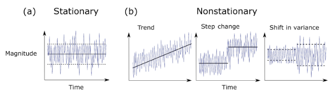
4. Stationarity: Statistical properties (mean, variance) don’t change over time
5. Autocorrelation: Correlation of a time series with its own past values
Introducing the Mauna Loa CO₂ Dataset
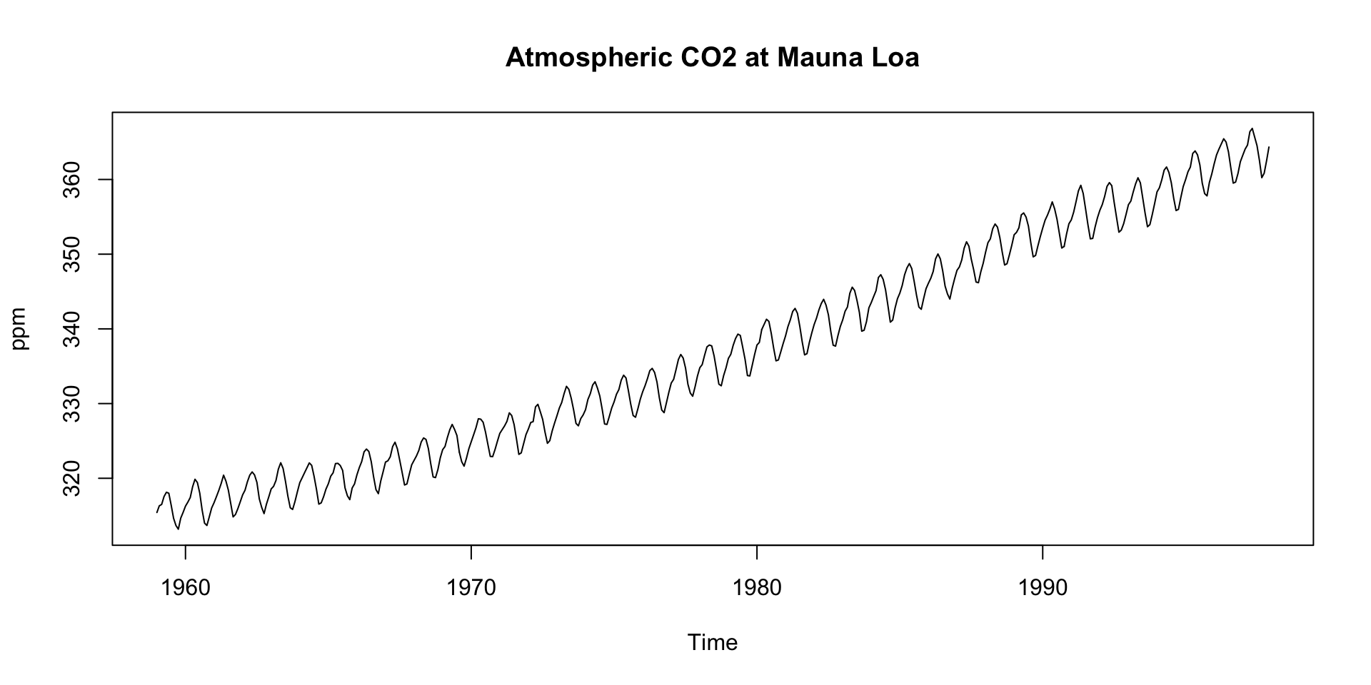
Mauna Loa CO₂ Dataset
The co2 dataset is a classic example of time series data. It contains monthly atmospheric CO₂ concentrations measured at the Mauna Loa Observatory in Hawaii.
co2 is a built-in dataset representing monthly CO₂ concentrations from 1959 onward.
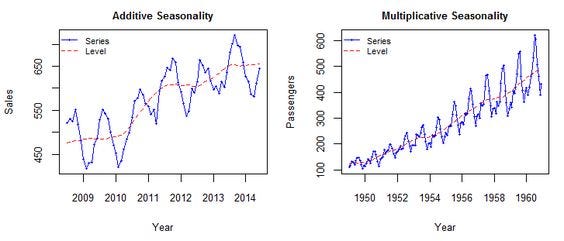
Use additive if seasonal variation is roughly constant.
Use multiplicative if it grows/shrinks with the trend.
Example
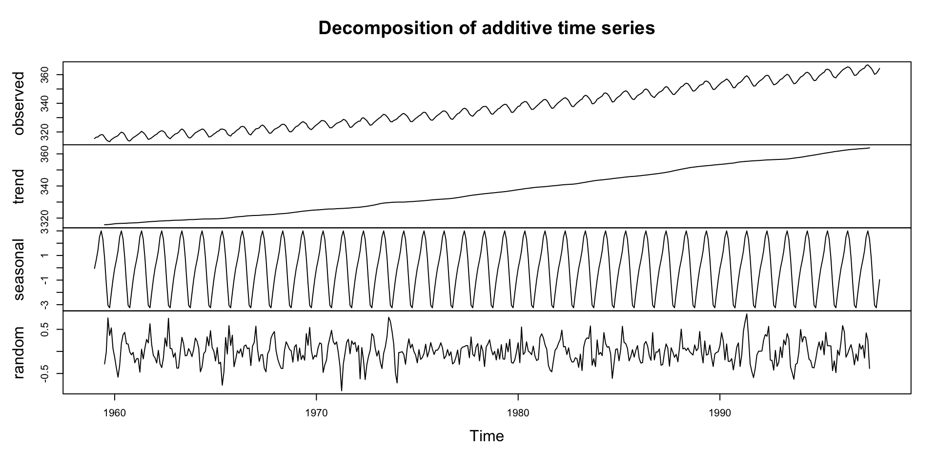
Why Decompose?
Trend: Are CO₂ levels increasing?
Seasonality: Are there predictable cycles each year?
Remainder: What’s left after we remove trend and season? (what is the randomness?)
Decompostion in R
The decompose() function in R can be used to perform this operation.
The decompose() function by default assumes that the time series is additive
decomp =decompose(co2, type ="additive")plot(decomp)
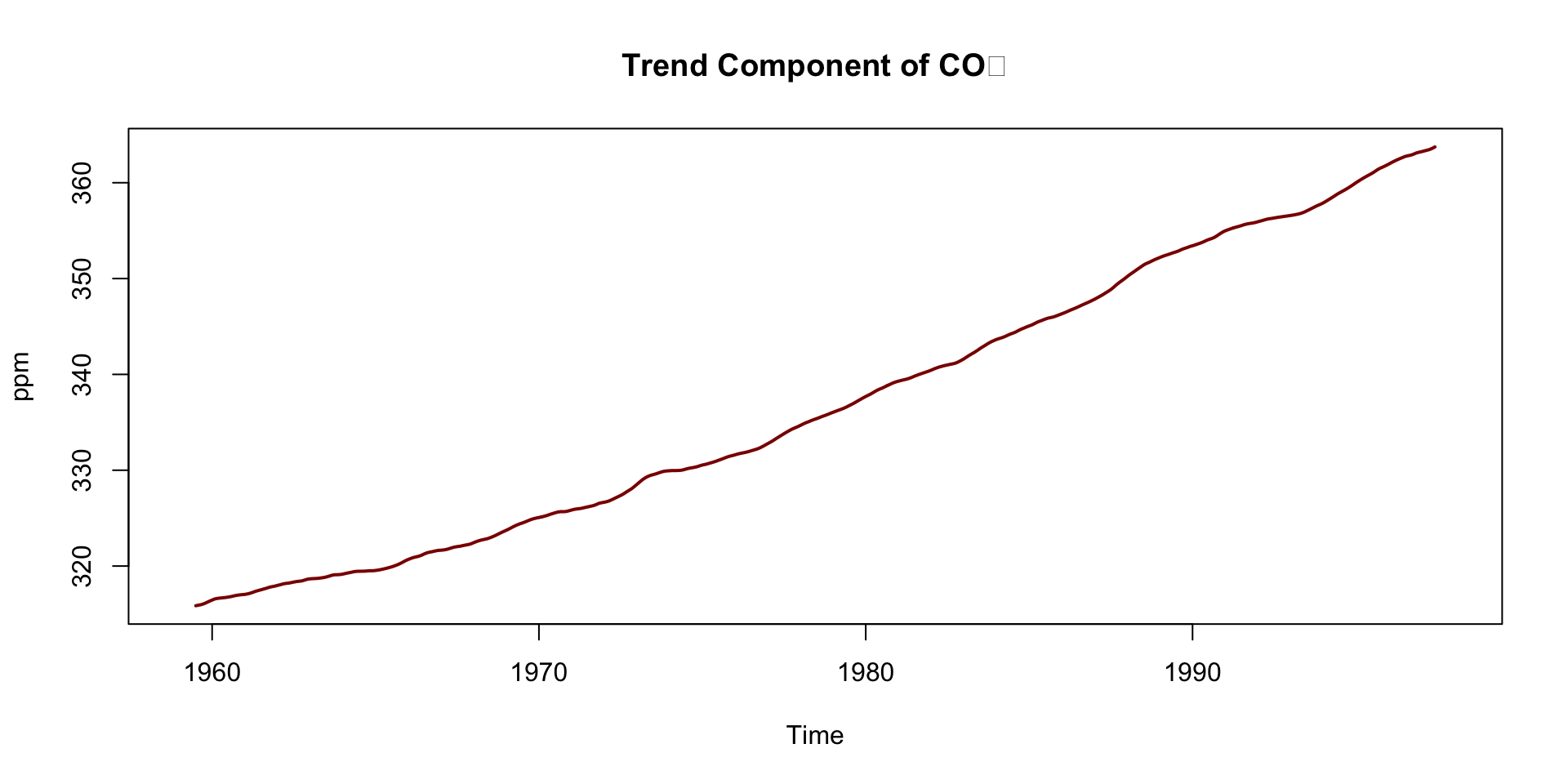
Deep Dive: Trend Component
plot(decomp$trend, main ="Trend Component of CO₂", ylab ="ppm", col ="darkred", lwd =2)
Steady upward slope from ~316 ppm in 1959 to ~365 ppm in the late 1990s
Captures the long-term forcing from human activity:
Fossil fuel combustion
Deforestation
This trend underpins climate change science — known as the Keeling Curve
Notice how the trend smooths short-term fluctuations
Interpreting the Trend
A linear model or loess smoother can also help quantify the trend:
co2_df <-data.frame(time =time(co2), co2 =as.numeric(co2))lm(as.numeric(co2) ~time(co2)) |>summary()#> #> Call:#> lm(formula = as.numeric(co2) ~ time(co2))#> #> Residuals:#> Min 1Q Median 3Q Max #> -6.0399 -1.9476 -0.0017 1.9113 6.5149 #> #> Coefficients:#> Estimate Std. Error t value Pr(>|t|) #> (Intercept) -2.250e+03 2.127e+01 -105.8 <2e-16 ***#> time(co2) 1.308e+00 1.075e-02 121.6 <2e-16 ***#> ---#> Signif. codes: 0 '***' 0.001 '**' 0.01 '*' 0.05 '.' 0.1 ' ' 1#> #> Residual standard error: 2.618 on 466 degrees of freedom#> Multiple R-squared: 0.9695, Adjusted R-squared: 0.9694 #> F-statistic: 1.479e+04 on 1 and 466 DF, p-value: < 2.2e-16
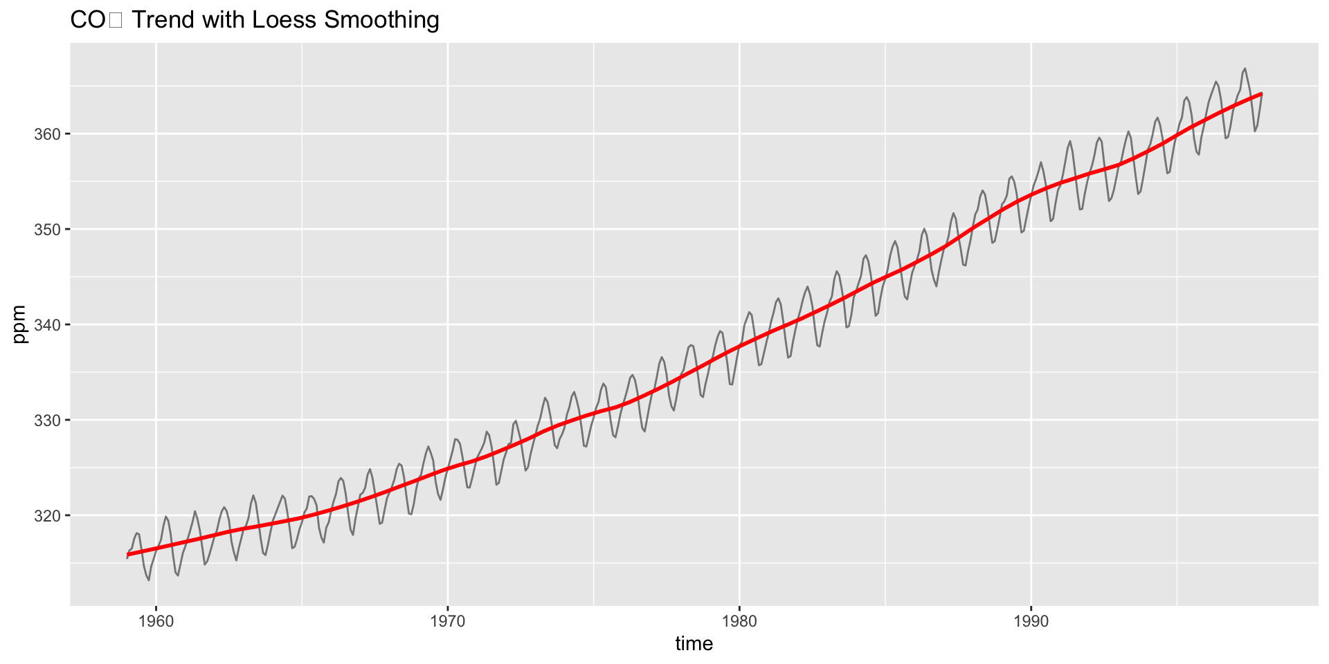
co2_df |>ggplot(aes(x = time, y = co2)) +geom_line(alpha =0.5) +geom_smooth(method ="loess", span =0.2, color ="red", se =FALSE) +labs(title ="CO₂ Trend with Loess Smoothing", y ="ppm")
Do you see acceleration in the rise over time?
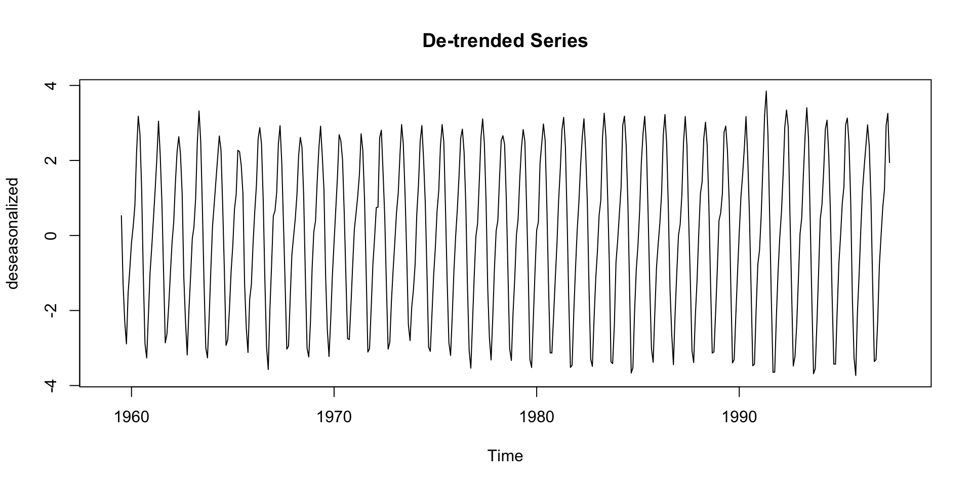
De-Trending
Detrending is the process of removing the trend component from a time series.
This can help for modeling the trend + residual only:
deseasonalized <- co2 - decomp$trendplot(deseasonalized, main ="De-trended Series")
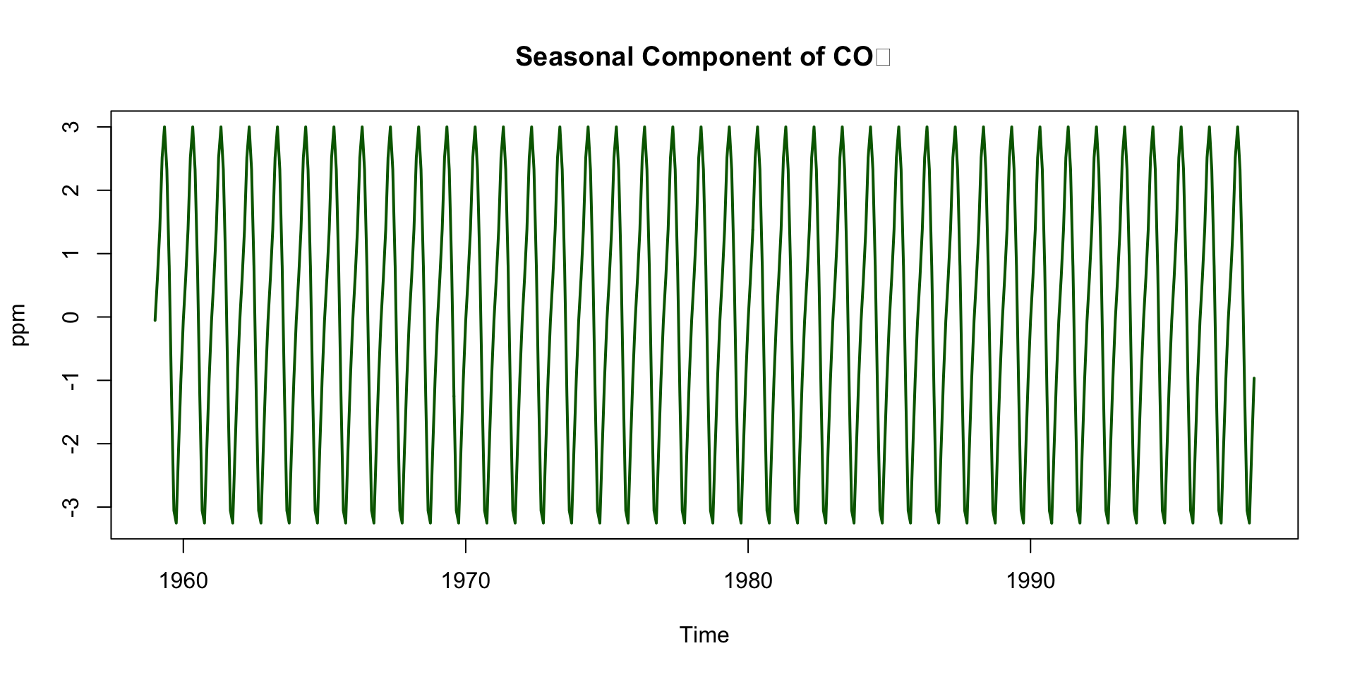
Deep Dive: Seasonal Component
plot(decomp$seasonal, main ="Seasonal Component of CO₂", ylab ="ppm", col ="darkgreen", lwd =2)
Repeats every 12 months
Peaks around May, drops in September–October
Driven by biospheric fluxes:
Photosynthesis during spring/summer → CO₂ drawdown
Decomposition and respiration in winter → CO₂ release
Seasonal Cycle is Northern Hemisphere-Dominated (Mauna Loa is in the Northern Hemisphere)
Northern Hemisphere contains more landmass and vegetation
So its biosphere exerts a stronger influence on global CO₂ than the Southern Hemisphere
This explains the pronounced seasonal cycle in the signal
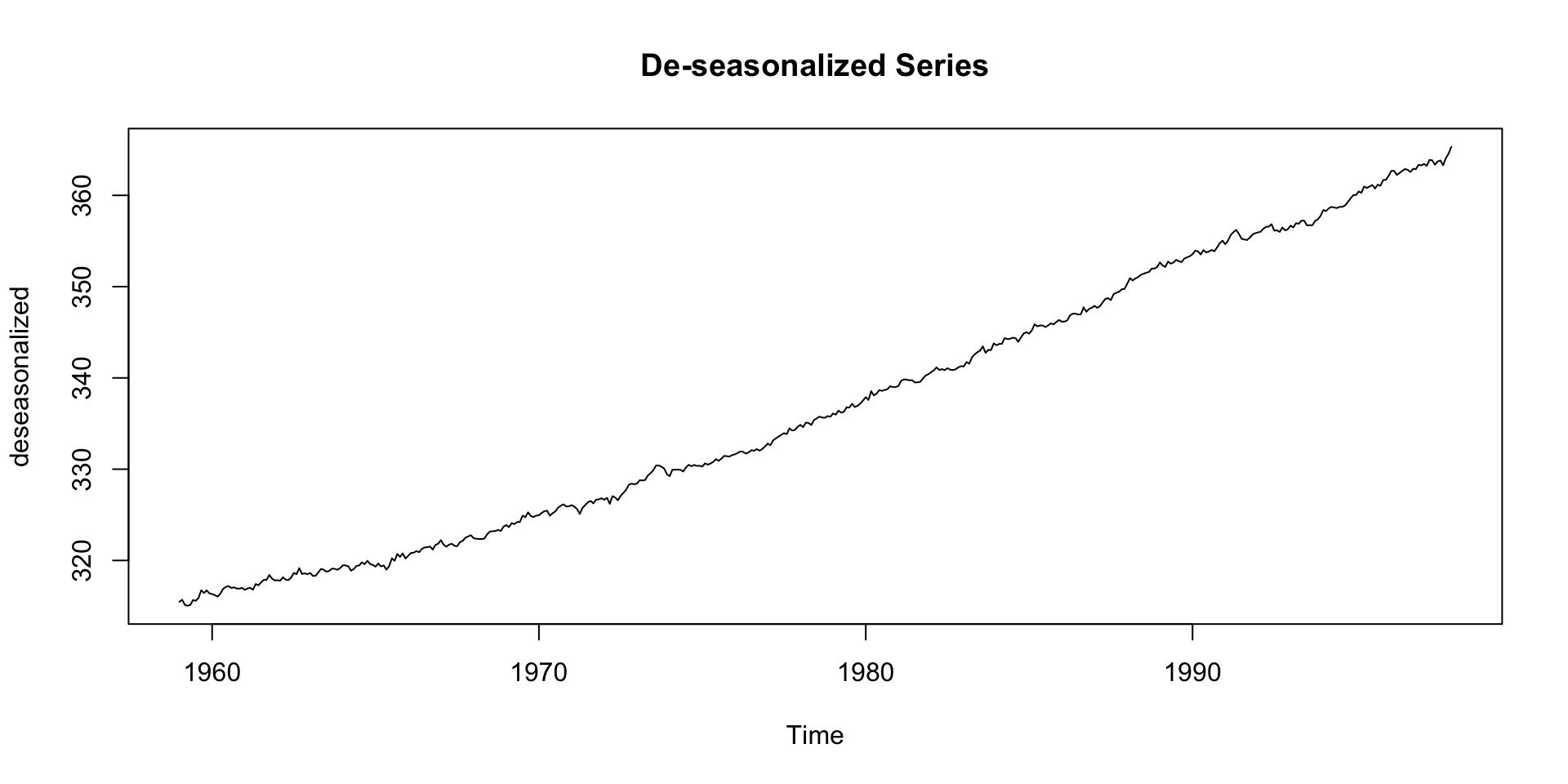
De-seasonalizing
This can help for modeling the seasonal + residual only:
deseasonalized <- co2 - decomp$seasonalplot(deseasonalized, main ="De-seasonalized Series")
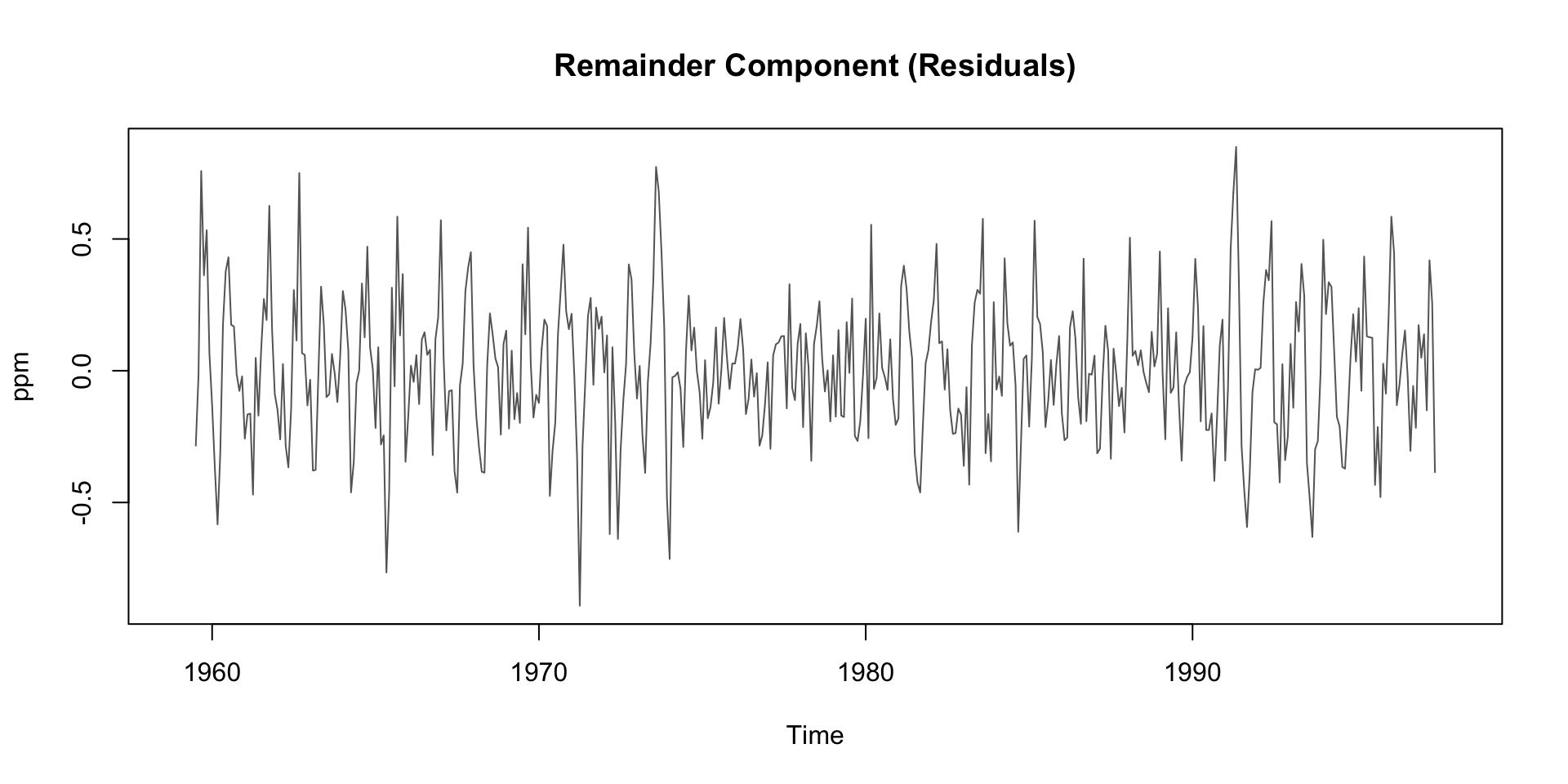
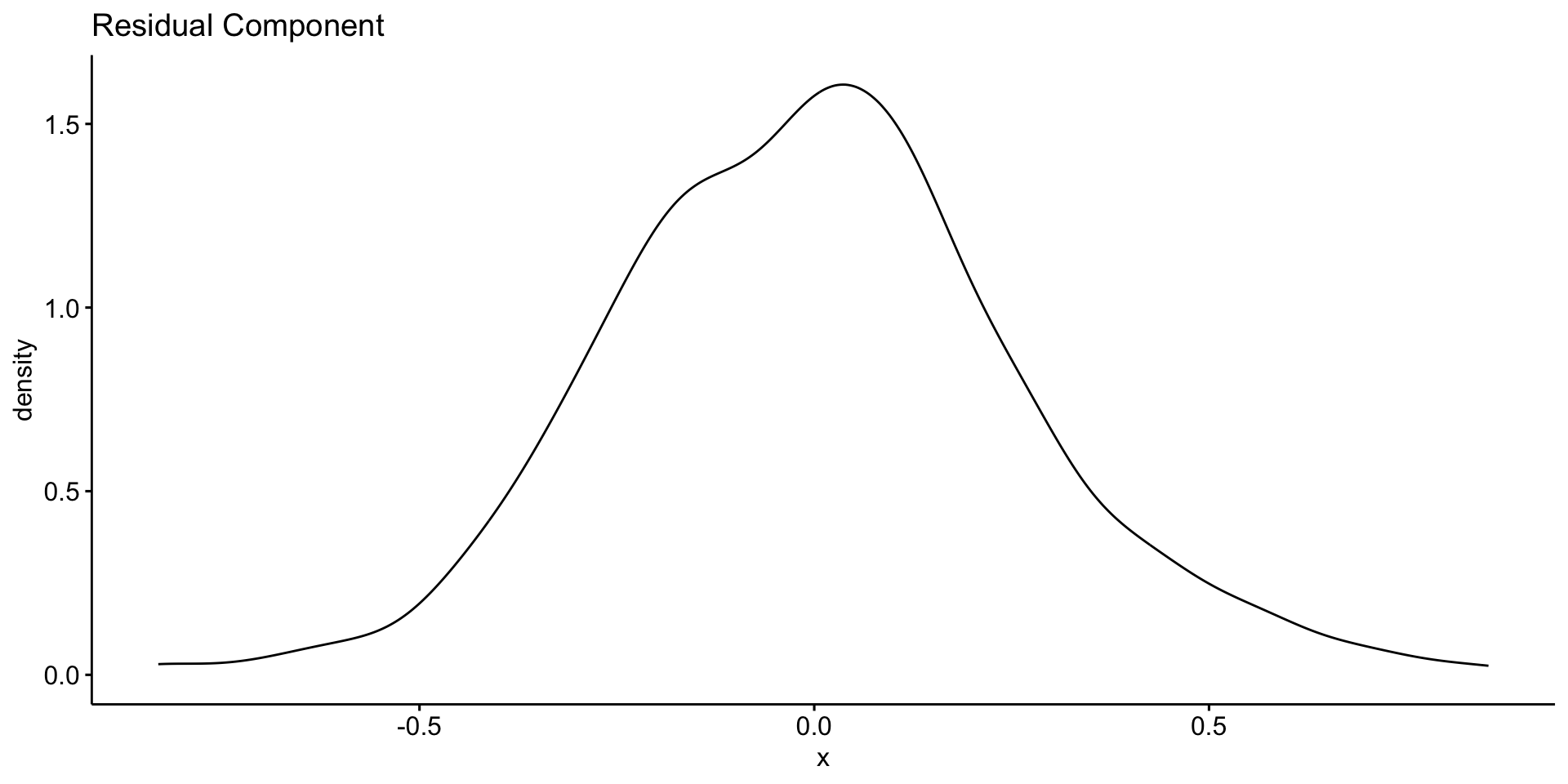
Deep Dive: Remainder Component
plot(decomp$random, main ="Remainder Component (Residuals)", ylab ="ppm", col ="gray40", lwd =1)
Residuals are the “leftover” part of the time series after removing trend and seasonality
Contains irregular, short-term fluctuations
Can be used to identify anomalies or outliers
Important for understanding noise in the data
Possible sources:
Volcanic activity (e.g. El Chichón, Mt. Pinatubo)
Measurement error
El Niño/La Niña events (which affect carbon flux)
Typically small amplitude: ±0.2 ppm
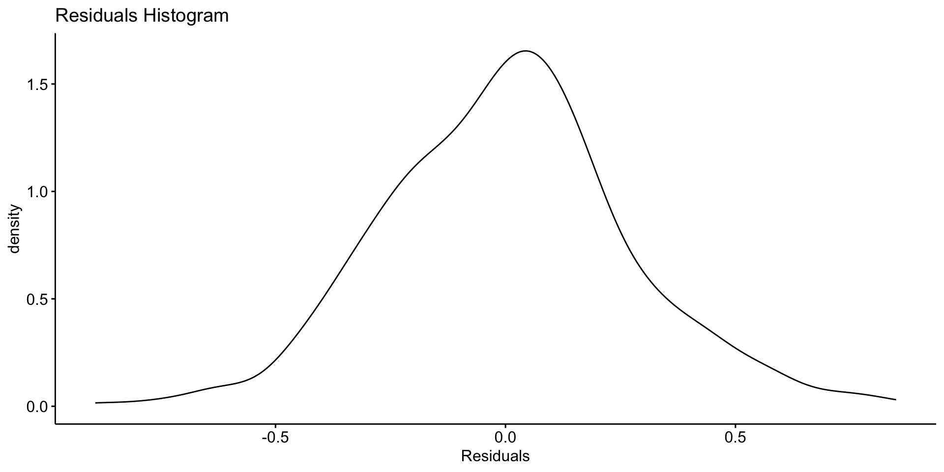
Asssessing Patterns in Error?
You might compute the standard deviation of the residuals to assess noise:
sd(na.omit(decomp$random))#> [1] 0.2651064
Or evaluate the residules like we did for Linear Modeling!
ggpubr::ggdensity(decomp$random, main ="Residuals Histogram", xlab ="Residuals")
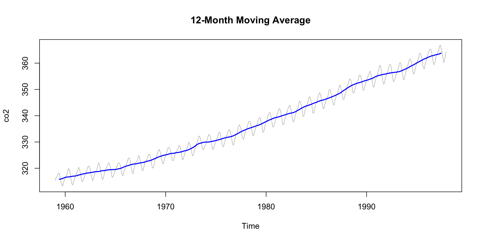
Smoothing to Remove Noise
If your data is noisy - and without usefull pattern - you can use a moving average to smooth it out.
The zoo package provides a convenient function for this that we have already seen in the COVID lab.
The rollmean() function from the zoo package is useful for this.
The k parameter specifies the window size for the moving average.
The align parameter specifies how to align the moving average with the original data (e.g., “center”, “left”, “right”).
The na.pad parameter specifies whether to pad the result with NA values.
co2_smooth <- zoo::rollmean(co2, k =12, align ="center", na.pad =TRUE)plot(co2, col ="grey", main ="12-Month Moving Average")lines(co2_smooth, col ="blue", lwd =2)
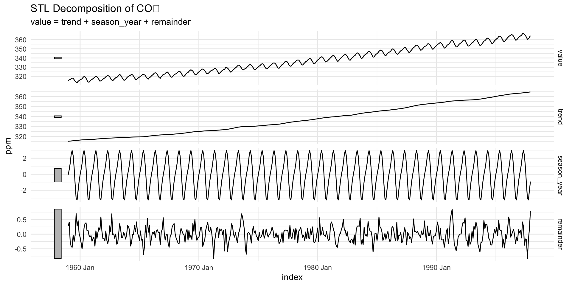
STL Decomposition (Loess-based)
STL (Seasonal-Trend decomposition using Loess) adapts to changing trend or seasonality over time
Doesn’t assume constant seasonal effect like decompose() does
Particularly valuable when working with:
Long datasets
Environmental time series affected by nonlinear changes
STL Decomposition (Loess-based)
stl() uses local regression (loess) to estimate the trend and seasonal components.
s.window = "periodic" specifies that the seasonal component is periodic.
Other options include
“none” (no seasonal component)
or a numeric value for the seasonal window size.
plot(decomp)
?stl(co2, s.window ="periodic") |>plot()#> Help on topic 'plot' was found in the following packages:#> #> Package Library#> graphics /Library/Frameworks/R.framework/Versions/4.4-arm64/Resources/library#> base /Library/Frameworks/R.framework/Resources/library#> #> #> Using the first match ...
Comparing Classical vs STL
Method
Assumes Constant Season?
Robust to Outliers?
Adaptive Smoothing?
decompose
✅ Yes
❌ No
❌ No
stl
✅ or 🔄 (customizable)
✅ Yes
✅ Yes
Recommendation: Use stl() for most real-world environmental time series.
Bringing It All Together
For the CO2 dataset, we can summarize the components of the time series:
Trend: A human fingerprint — atmospheric CO₂ continues to rise year over year
Seasonality: Driven by biospheric rhythms with not multiplicative gains
Remainder: Small, but potentially rich with short-term signals
Understanding these components lets us:
✅ Track long-term progress
✅ Forecast future CO₂
✅ Communicate patterns clearly to policymakers
Time Series in the Tidyverse: tsibble / feasts
tsibble is a tidy data frame for time series data. It extends the tibble class to include time series attributes.
Compatible with dplyr, ggplot2
feasts provides functions for time series analysis and visualization.
co2_tbl <-as_tsibble(co2)head(co2_tbl)#> # A tsibble: 6 x 2 [1M]#> index value#> <mth> <dbl>#> 1 1959 Jan 315.#> 2 1959 Feb 316.#> 3 1959 Mar 316.#> 4 1959 Apr 318.#> 5 1959 May 318.#> 6 1959 Jun 318
Decomposing with feasts
feasts provides:
a STL() function for seasonal decomposition.
components() extracts the components of the decomposition.
gg_season() and gg_subseries() visualize seasonal patterns.
gg_lag() visualizes autocorrelation and lagged relationships.
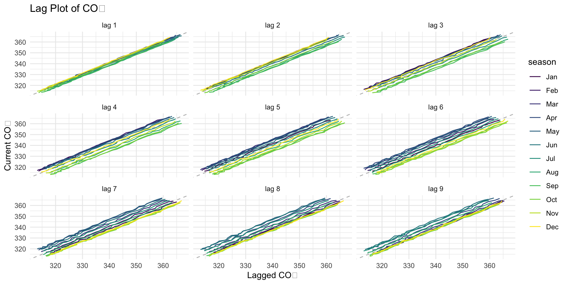
A lag plot is a scatterplot of a time series against itself, but with a time shift (or “lag”) applied to one of the series.
It helps us visualize the relationship between current and past values of a time series.
📦 Here’s the simple idea:
You take your CO₂ measurements over time.
Then you make a graph where you plot today’s CO₂ (on the Y-axis)…
…against CO₂ from a few months ago (on the X-axis).
This shows you if the past helps predict the present!
📊 If it makes a curvy shape or a line…
…that means there’s a pattern! Your data remembers what happened before — like a smart friend who learns from their past.
But if the dots look like a big messy spaghetti mess that means the data is random, with no memory of what happened before.
gg_lag()
🧠 Why this is useful:
It helps us see if there are patterns in the data.
It helps us understand how past values affect current values.
It helps us decide if we can use this data to make predictions in the future.
co2_tbl |>gg_lag() +labs(title ="Lag Plot of CO₂", x ="Lagged CO₂", y ="Current CO₂") +theme_minimal()
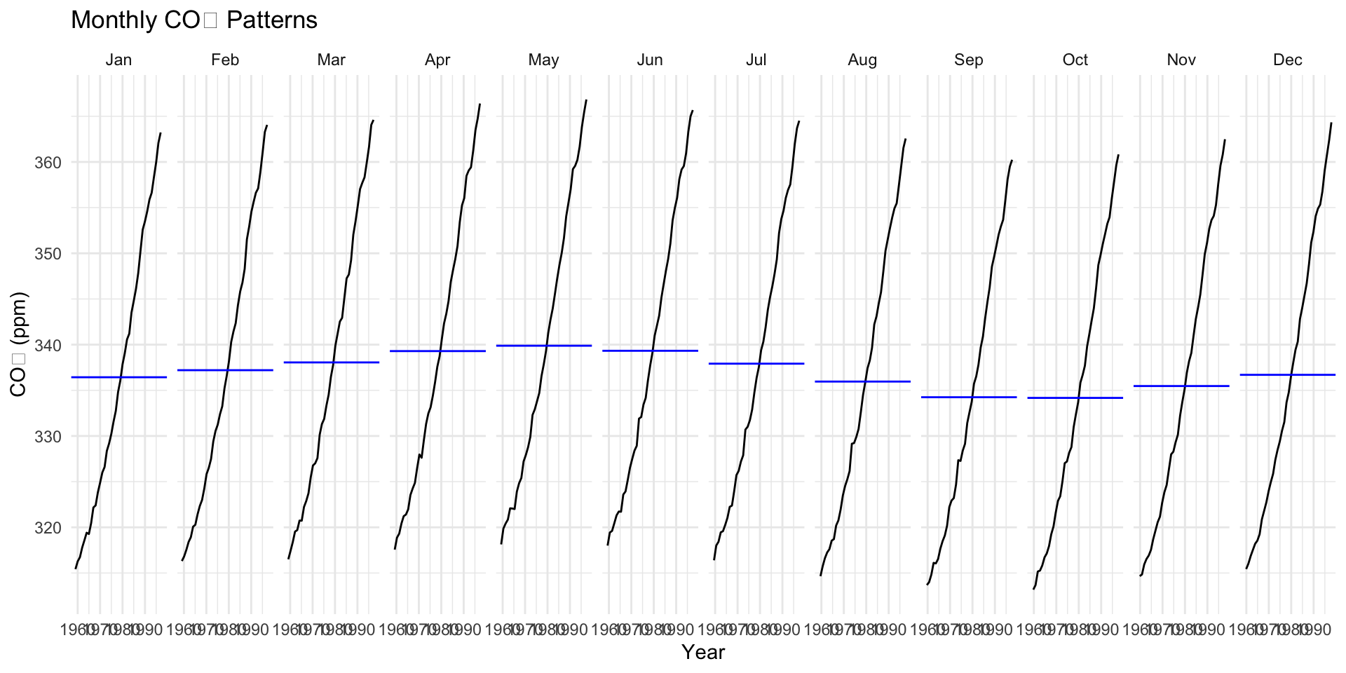
gg_subseries
Imagine the co2 dataset as a big collection of monthly CO₂ data from Mauna Loa. Each month is a group, and each year is a new object
Now, we want to see how each month behaves across the years, so we can spot if January always has higher or lower CO₂ levels, for example.
📊 What this does:
Each month: A different color shows up for each month (like January in blue, February in red, etc.)
Lines: You see the CO₂ values for each month over different years. For example, you might notice that CO₂ levels tend to be higher in the spring and lower in the fall.
🧠 Why this is useful:
We can spot seasonal trends: Does CO₂ rise in the winter? Or fall in the summer?
We can also compare months across the years: Is January more or less CO₂-heavy compared to other months?
gg_subseries()
gg_subseries(co2_tbl) +labs(title ="Monthly CO₂ Patterns", y ="CO₂ (ppm)", x ="Year") +theme_minimal()
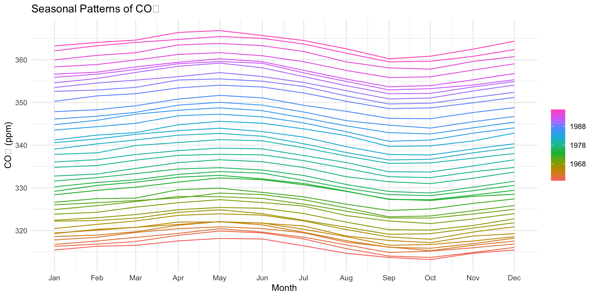
gg_season
Think of gg_season() like a way to look at a yearly picture of CO₂ and see if the Earth follows a seasonal rhythm.
It makes the changes in CO₂ easy to spot when you look at months side-by-side.
📊 What this does:
It shows you how CO₂ changes during each month of the year, but it puts all the years together, so you can see if the same thing happens every year in January, February, and so on.
🧠 Why this is useful:
You’ll see a smooth curve for each month. Each curve shows how CO₂ goes up and down each year in the same pattern.
gg_season
gg_season(co2_tbl) +labs(title ="Seasonal Patterns of CO₂", y ="CO₂ (ppm)", x ="Month") +theme_minimal()
Bonus: Interactive Plotting
In last weeks demo, we used plotly to generate an interactive plot of the hyperparameter tuning process.
You can use the plotly package to add interactivity to your ggplots directly with ggplotly()!
library(plotly)co2_plot <- co2_tbl |>autoplot() +geom_line(color ="steelblue") +labs(title ="Interactive CO₂ Time Series", x ="Date", y ="ppm")
Bonus: Interactive Plotting
ggplotly(co2_plot)
Forecasting:
Forecasting with two distinct models (1) ARIMA (2) Prophet
Understanding modeltime + tidymodels integration
Forecasting Process for time series
Toy Example: River Time Series & ARIMA
Let’s say we’re watching how much water flows in a river every day:
Monday: 50 cfs
Tuesday: 60 cfs
Wednesday: 70 cfs
We want to guess tomorrow’s flow.
1. AutoRegressive (AR)
This means: “Look at yesterday and the day before!”
If flow has been going up each day, AR says: ** “Tomorrow might go up again …” **
It’s like the river has a pattern.
2. Integrated (I)
Sometimes the flow just keeps climbing — like during a spring snowmelt!
To help ARIMA think better, we subtract yesterday’s number from today’s.
This makes the numbers more steady so ARIMA can do its magic.
3. Moving Average (MA)
The river sometimes gets a surprise flux (like a big rainstorm 🌧️).
MA looks at those surprises and helps smooth them out.
So if it rained two days ago, MA might say: “Don’t expect another surprise tomorrow.”
Put It All Together: AR + I + MA = ARIMA
AR: Uses the river’s memory (trend)
I: Calms the sturcutral components (season)
MA: Handles noisy surprises (noise)
Now we can forecast tomorrow’s flow!
ARIMA
The basics of a ARIMA (AutoRegressive Integrated Moving Average) Model include:
AR: AutoRegressive part (past values):
AR(1) = current value depends on the previous value
AR(2) = current value depends on the previous two values
I: Integrated part (differencing to make data stationary)
Differencing removes trends and seasonality
e.g., diff(co2, lag = 12) removes annual seasonality
MA: Moving Average part (past errors)
MA(1) = current value depends on the previous error
MA(2) = current value depends on the previous two errors
p, d, q: Parameters for AR, I, and MA
p = number of lagged values (AR)
d = number of differences (I)
q = number of lagged errors (MA)
AIC
The AIC metric helps choose between models/parameters:
It rewards:
Good predictions
Simplicity
It punishes:
Complexity (too many parameters)
Overfitting (fitting noise instead of the trend)
Lower AIC = better model
A Simple Forecasting Example
auto.arima() is a function from the forecast package that automatically selects the best ARIMA model for your data accoridning toe to the AICc criterion.
The AICc (Akaike Information Criterion corrected) is a measure of the relative quality of statistical models for a given dataset.
It is used to compare different models and select the one that best fits the data while penalizing for complexity.
The auto.arima() function will automatically select the best parameters (p,d,q) based on the AICc criterion.
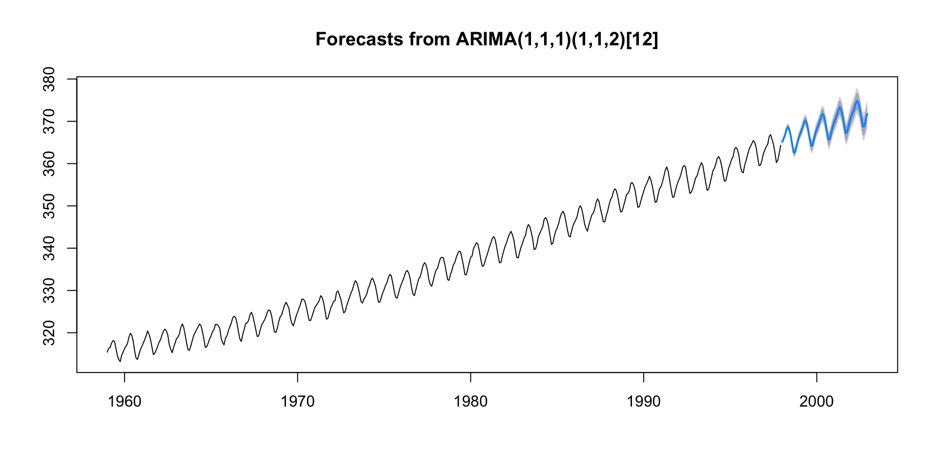
library(forecast)co2_arima <-auto.arima(co2)summary(co2_arima)#> Series: co2 #> ARIMA(1,1,1)(1,1,2)[12] #> #> Coefficients:#> ar1 ma1 sar1 sma1 sma2#> 0.2569 -0.5847 -0.5489 -0.2620 -0.5123#> s.e. 0.1406 0.1204 0.5880 0.5701 0.4819#> #> sigma^2 = 0.08576: log likelihood = -84.39#> AIC=180.78 AICc=180.97 BIC=205.5#> #> Training set error measures:#> ME RMSE MAE MPE MAPE MASE#> Training set 0.01742092 0.287159 0.2303994 0.005073769 0.06845665 0.1819636#> ACF1#> Training set -0.002858162
Forecasting with ARIMA
The forecast() function is used to generate forecasts from the fitted ARIMA model.
The h argument specifies the number of periods to forecast into the future.
co2_forecast <-forecast(co2_arima, h =60)plot(co2_forecast)
🔢 ARIMA(1,1,1)(1,1,2)[12]
ARIMA Notation can be broken into two parts:
1. Non-seasonal part: ARIMA(1, 1, 1)
This is the “regular” ARIMA: - AR(1): One autoregressive term — the model looks at one lag of the time series.
I(1): One differencing — the model uses the change in values instead of raw values to make the series more stationary.
MA(1): One moving average term — the model corrects using one lag of the error term.
2. Seasonal part: (1, 1, 2)[12]
This is the seasonal pattern — repeated every 12 time units (like months in a year):
SAR(1): One seasonal autoregressive term — it uses the value from 12 time steps ago.
SI(1): One seasonal difference — subtracts the value from 12 steps ago to remove seasonal patterns.
SMA(2): Two seasonal moving average terms — uses errors from 12 and 24 time steps ago.
[12]: This is the seasonal period, i.e., it’s a yearly pattern with monthly data.
🔢 ARIMA(1,1,1)(1,1,2)[12]
Hey, ARIMA please…
“Model the data using a mix of its last value, the last error, and their seasonal versions from 12 months ago — but first difference it once to remove trend and once seasonally to remove yearly patterns.”
Note
ARIMA modeling works well when data is stationary. - Stationarity means the statistical properties of the series (mean, variance) do not change over time. - Non-stationary data can lead to unreliable forecasts and misleading results.
Prophet
Prophet is an open-source tool for forecasting time series data.
Developed by Facebook (Meta)
Designed for analysts and data scientists
Handles missing data, outliers, and seasonality
Key Features of Prophet
✅ Additive Model: Trend + Seasonality + Holidays + Noise
✅ Automatic Changepoint Detection
✅ Support for Custom Holidays & Events
✅ Flexible Seasonality (daily/weekly/yearly)
✅ Easy-to-use API in R and Python
Prophet’s Model Structure
Prophet decomposes time series into components:
\[ y(t) = g(t) + s(t) + h(t) + ε(t) \]
g(t): Trend (linear or logistic growth)
s(t): Seasonality (Fourier series)
h(t): Holiday effects
ε(t): Error term (noise)
📌 Assumes additive components by default; multiplicative also possible
A Simple Forecasting Example
Your time series must have: (1) ds column (date/timestamp) (2) y column (value to forecast)
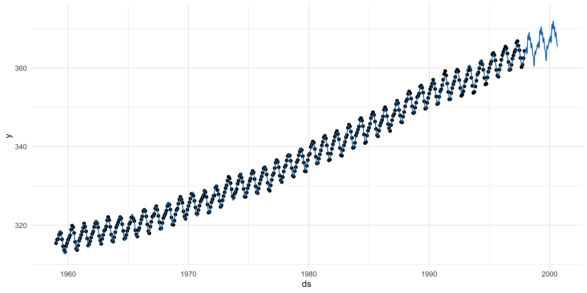
library(prophet)prophet_mod <- tsibble::as_tsibble(co2) |># prophet requires ds and y columns dplyr::rename(ds = index, y = value) |>prophet()
# Make future dataframe and predictfuture <-make_future_dataframe(prophet_mod, periods =1000)forecast <-predict(prophet_mod, future)# Plot the forecastplot(prophet_mod, forecast) +theme_minimal()
Pros / Cons
Feature
ARIMA
Prophet
Statistical rigor
Based on strong statistical theory; well-studied
Intuitive, decomposable model (trend + seasonality + events)
Interpretability
Clear interpretation of AR, MA, differencing terms
Model Spec: arima_reg()/prophet_reg()/prophet_boost() <– This sets up your general model algorithm and key parameters
Model Mode: mode = "regression"/mode = "classification" <– This sets the model mode to regression or classification (timeseries is always regression!)
Set Engine: set_engine("auto_arima")/set_engine("prophet") / <– This selects the specific package-function to use, you can add any function-level arguments here.
modeltime_table() does some basic checking to ensure all models are fit and organized into a scalable structure called a “Modeltime Table” that is used as part of our forecasting workflow.
It’s expected that tuning and parameter selection is performed prior to incorporating into a Modeltime Table.
If you try to add an unfitted model, the modeltime_table() will complain (throw an informative error) saying you need to fit() the model.
5. Calibrate the Models …
Use modeltime_calibrate() to evaluate the models on the test set.
Calibrating adds a new column, .calibration_data, with the test predictions and residuals inside.
Calibration builds confidence intervals and accuracy metrics
Calibration Data is the predictions and residuals that are calculated from out-of-sample data.
After calibrating, the calibration data follows the data through the forecasting workflow.
Testing Forecast & Accuracy Evaluation
There are 2 critical parts to an evaluation.
Evaluating the Test (Out of Sample) Accuracy
Visualizing the Forecast vs Test Data Set
Accuracy
modeltime_accuracy() collects common accuracy metrics using yardstick functions:
MAE - Mean absolute error, mae()
MAPE - Mean absolute percentage error, mape()
MASE - Mean absolute scaled error, mase()
SMAPE - Symmetric mean absolute percentage error, smape()
RMSE - Root mean squared error, rmse()
RSQ - R-squared, rsq()
modeltime_accuracy(calibration_table) |>arrange(mae)#> # A tibble: 6 × 9#> .model_id .model_desc .type mae mape mase smape rmse rsq#> <int> <chr> <chr> <dbl> <dbl> <dbl> <dbl> <dbl> <dbl>#> 1 1 ARIMA(1,1,1)(2,1,2)[12] Test 0.810 0.224 0.687 0.224 0.967 0.973#> 2 2 ARIMA(1,1,1)(0,1,1)[12] Test 0.885 0.244 0.750 0.245 1.05 0.969#> 3 3 PROPHET Test 1.06 0.295 0.899 0.294 1.16 0.986#> 4 4 PROPHET Test 1.06 0.295 0.899 0.294 1.16 0.986#> 5 5 ETS(M,A,A) Test 1.48 0.409 1.25 0.410 1.71 0.958#> 6 6 EARTH Test 1.89 0.526 1.61 0.526 2.25 0.499
Forecast
Use modeltime_forecast() to generate forecasts for the next 120 months (10 years).
Use plot_modeltime_forecast() to visualize the forecasts.
(forecast <- calibration_table |>modeltime_forecast(h ="60 months", new_data = testing,actual_data = co2_tbl) )#> # Forecast Results#> #> # A tibble: 828 × 7#> .model_id .model_desc .key .index .value .conf_lo .conf_hi#> <int> <chr> <fct> <date> <dbl> <dbl> <dbl>#> 1 NA ACTUAL actual 1959-01-01 315. NA NA#> 2 NA ACTUAL actual 1959-02-01 316. NA NA#> 3 NA ACTUAL actual 1959-03-01 316. NA NA#> 4 NA ACTUAL actual 1959-04-01 318. NA NA#> 5 NA ACTUAL actual 1959-05-01 318. NA NA#> 6 NA ACTUAL actual 1959-06-01 318 NA NA#> 7 NA ACTUAL actual 1959-07-01 316. NA NA#> 8 NA ACTUAL actual 1959-08-01 315. NA NA#> 9 NA ACTUAL actual 1959-09-01 314. NA NA#> 10 NA ACTUAL actual 1959-10-01 313. NA NA#> # ℹ 818 more rows
Vizualize
plot_modeltime_forecast(forecast)
Refit to Full Dataset & Forecast Forward
The final step is to refit the models to the full dataset using modeltime_refit() and forecast them forward.