Basic Use
Mike Johnson
Lynker, NOAA-Affiliatebasic_use.Rmd
library(hydrofabric3D)The goal of hydrofabric3D is to generate DEM-based cross sections for hydrographic networks.
Installation
You can install the development version of hydrofabric3D from GitHub with:
# install.packages("devtools")
devtools::install_github("mikejohnson51/hydrofabric3D")
Example
This is a basic example which shows you how to cut cross sections for a network.
Define Network
library(hydrofabric3D)
library(dplyr)
#>
#> Attaching package: 'dplyr'
#> The following objects are masked from 'package:stats':
#>
#>     filter, lag
#> The following objects are masked from 'package:base':
#>
#>     intersect, setdiff, setequal, union

(net = linestring %>%
  mutate(bf_width = exp(0.700    + 0.365* log(totdasqkm))))
#> Simple feature collection with 325 features and 5 fields
#> Geometry type: LINESTRING
#> Dimension:     XY
#> Bounding box:  xmin: 77487.09 ymin: 890726.5 xmax: 130307.4 ymax: 939129.8
#> Projected CRS: NAD83 / Conus Albers
#> # A tibble: 325 × 6
#>    nhdplus_comid                       geometry  comid totdasqkm dist_m bf_width
#>  * <chr>                       <LINESTRING [m]>  <dbl>     <dbl>  <dbl>    <dbl>
#>  1 101           (128525.6 892408.3, 128565.7 … 1.01e2  7254.    3.25e3   51.7
#>  2 24599575      (128084.7 892952.4, 128525.6 … 2.46e7  7249.    7.00e2   51.6
#>  3 1078635       (127687.6 893270.4, 127799.7 … 1.08e6  7248.    5.22e2   51.6
#>  4 1078637       (124942.8 893959.6, 124948.2 … 1.08e6    68.2   4.17e3    9.41
#>  5 1078639       (125523.1 892528, 125657.3 89… 1.08e6  7180.    2.76e3   51.5
#>  6 1078577       (123219.9 902292.8, 123233.5 … 1.08e6    19.8   9.91e3    5.99
#>  7 1078575       (121975.5 909050.8, 122028.9 … 1.08e6    41.3   1.87e4    7.83
#>  8 1078657       (124263.8 892410.4, 124420.6 … 1.08e6  7179.    1.66e3   51.5
#>  9 1078663       (125628.9 892216, 125555.7 89… 1.08e6     0.099 7.54e2    0.866
#> 10 1078643       (124248.1 892440.7, 124263.8 … 1.08e6  7178.    3.41e1   51.5
#> # ℹ 315 more rows


plot(net$geometry)
Cut cross sections
(transects = cut_cross_sections(net = net,
                         id = "comid",
                         cs_widths = pmax(50, net$bf_width * 7),
                         num = 10) )
#> Smoothing
#> Densifying
#> Cutting
#> Formating
#> Warning: st_centroid assumes attributes are constant over geometries
#> Simple feature collection with 2275 features and 7 fields
#> Geometry type: LINESTRING
#> Dimension:     XY
#> Bounding box:  xmin: 77473.82 ymin: 890553.2 xmax: 130336.7 ymax: 939136.7
#> Projected CRS: NAD83 / Conus Albers
#> # A tibble: 2,275 × 8
#>    ds_distance cs_measure    hy_id cs_widths                      geometry cs_id
#>          <dbl>      <dbl>    <dbl>     <dbl>              <LINESTRING [m]> <int>
#>  1       367.        11.2      101      362. (128409.2 892046.4, 128768.1…     1
#>  2       818.        25.0      101      362. (128553.4 891572.7, 128890.1…     2
#>  3      1242.        38.0      101      362. (128838.4 891220.8, 129145.3…     3
#>  4      1629.        49.8      101      362. (129198.3 890891.1, 129319.4…     4
#>  5      1962.        60.0      101      362. (129590.7 891044.8, 129463.9…     5
#>  6      2241.        68.5      101      362. (129732.4 891134.4, 129742 8…     6
#>  7      2487.        76.0      101      362. (129719.7 891083.8, 130016.4…     7
#>  8      2813.        86.0      101      362. (129907.8 891136.4, 130208.7…     8
#>  9      3260.        99.6      101      362. (130254.3 890553.2, 130336.7…     9
#> 10        77.8       11.1 24599575      362. (127993.3 892778.2, 128274.1…     1
#> # ℹ 2,265 more rows
#> # ℹ 2 more variables: lengthm <dbl>, sinuosity <dbl>

plot(transects$geometry)
Define Cross section points
(pts = cross_section_pts(transects,
                        dem = "/vsicurl/https://prd-tnm.s3.amazonaws.com/StagedProducts/Elevation/1/TIFF/USGS_Seamless_DEM_1.vrt"))
#> Simple feature collection with 23416 features and 11 fields
#> Geometry type: POINT
#> Dimension:     XY
#> Bounding box:  xmin: 77475.72 ymin: 890567.9 xmax: 130333.3 ymax: 939134.7
#> Projected CRS: NAD83 / Conus Albers
#> # A tibble: 23,416 × 12
#>    hy_id cs_id pt_id     Z lengthm relative_distance ds_distance cs_measure
#>    <dbl> <int> <int> <dbl>   <dbl>             <dbl>       <dbl>      <dbl>
#>  1   101     1     1  42.2    362.               0          367.       11.2
#>  2   101     1     2  42.1    362.              32.9        367.       11.2
#>  3   101     1     3  42.5    362.              65.7        367.       11.2
#>  4   101     1     4  42.4    362.              98.6        367.       11.2
#>  5   101     1     5  40.2    362.             131.         367.       11.2
#>  6   101     1     6  40.2    362.             164.         367.       11.2
#>  7   101     1     7  36.2    362.             197.         367.       11.2
#>  8   101     1     8  39.9    362.             230.         367.       11.2
#>  9   101     1     9  39.7    362.             263.         367.       11.2
#> 10   101     1    10  40.5    362.             296.         367.       11.2
#> # ℹ 23,406 more rows
#> # ℹ 4 more variables: cs_widths <dbl>, sinuosity <dbl>, points_per_cs <dbl>,
#> #   geometry <POINT [m]>
Classify Cross section points
(classified_pts = classify_points(pts))
#> Simple feature collection with 23416 features and 7 fields
#> Geometry type: POINT
#> Dimension:     XY
#> Bounding box:  xmin: 77475.72 ymin: 890567.9 xmax: 130333.3 ymax: 939134.7
#> Projected CRS: NAD83 / Conus Albers
#> # A tibble: 23,416 × 8
#>    hy_id cs_id pt_id     Z relative_distance cs_widths class
#>    <dbl> <int> <int> <dbl>             <dbl>     <dbl> <chr>
#>  1   101     1     1  42.2               0        362. left_bank
#>  2   101     1     2  42.2              32.9      362. left_bank
#>  3   101     1     3  42.3              65.7      362. left_bank
#>  4   101     1     4  41.7              98.6      362. channel
#>  5   101     1     5  40.9             131.       362. channel
#>  6   101     1     6  38.9             164.       362. channel
#>  7   101     1     7  36.2             197.       362. bottom
#>  8   101     1     8  38.6             230.       362. channel
#>  9   101     1     9  40.0             263.       362. right_bank
#> 10   101     1    10  41.2             296.       362. right_bank
#> # ℹ 23,406 more rows
#> # ℹ 1 more variable: geometry <POINT [m]>
Explore!
library(ggplot2)

ggplot(data = filter(classified_pts, hy_id == 101) ) +
  geom_line(aes(x = relative_distance, y = Z)) +
  geom_point(aes(x = relative_distance, y = Z, color = class)) +
  facet_wrap(~cs_id, scales = "free") +
  theme_minimal() +
  theme(legend.position = "bottom")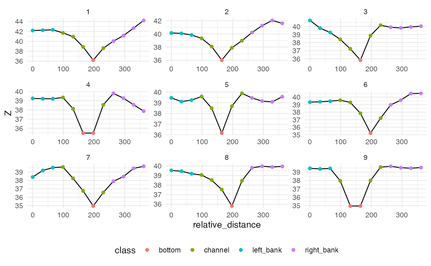
Time to get 2275 transects and 23416 classified points …
system.time({
  cs = net %>%
  cut_cross_sections(id = "comid",
                     cs_widths = pmax(50, net$bf_width * 7),
                     num = 10) %>%
  cross_section_pts(dem = '/vsicurl/https://prd-tnm.s3.amazonaws.com/StagedProducts/Elevation/1/TIFF/USGS_Seamless_DEM_1.vrt') %>%
  classify_points()
})
#> Smoothing
#> Densifying
#> Cutting
#> Formating
#> Warning: st_centroid assumes attributes are constant over geometries
#>    user  system elapsed
#>  18.788   0.339  21.747