NOAA OWP Cross Section Generator

Introduction

The need to cut transects of elevation along a set of lines (e.g. river or road networks) is a fairly common task with an unsatisfying number of off the shelf solutions. For our particular need at OWP we need to cut cross sections across the entire CONUS river network to provide much needed information to flood mapping and hydrologic modeling tasks. This document shows some of the initial efforts towards doing this at that scale. For small sets of cross sections the tools developed by Rich McDonald (e.g. nhdplusTools::get_xs_point) should be preferred.

Prep Network

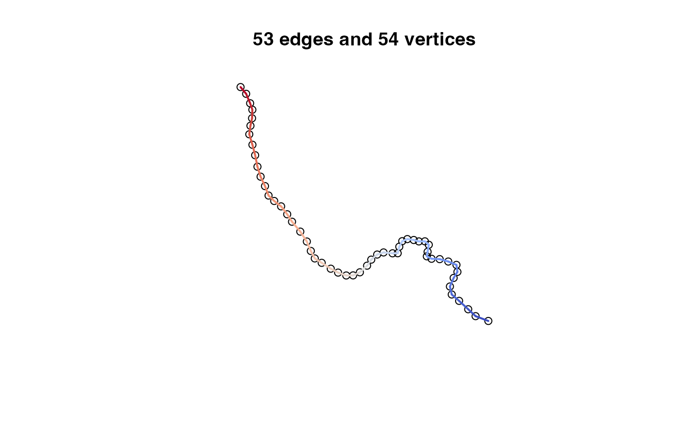
Here we are loading the Upper Tributary of COMID 101. In total there are 325 flowlines with a total length of 942.3 km.

We also prescribe a floodplain width by computing the estimated bank full width (from literature based power-law) and multiplying it by 5. This assumes 2 parts left-bank, 1 part in channel (bank full), 2 parts right-bank. This will be important latter!

flood_plain_sections = 5
network = linestring %>% 
  # https://agupubs.onlinelibrary.wiley.com/doi/full/10.1002/2013WR013916
  mutate(bf_width = exp(0.700    + 0.365* log(totdasqkm)),
         cs_width = flood_plain_sections * bf_width)

Algorithm Walk Through:

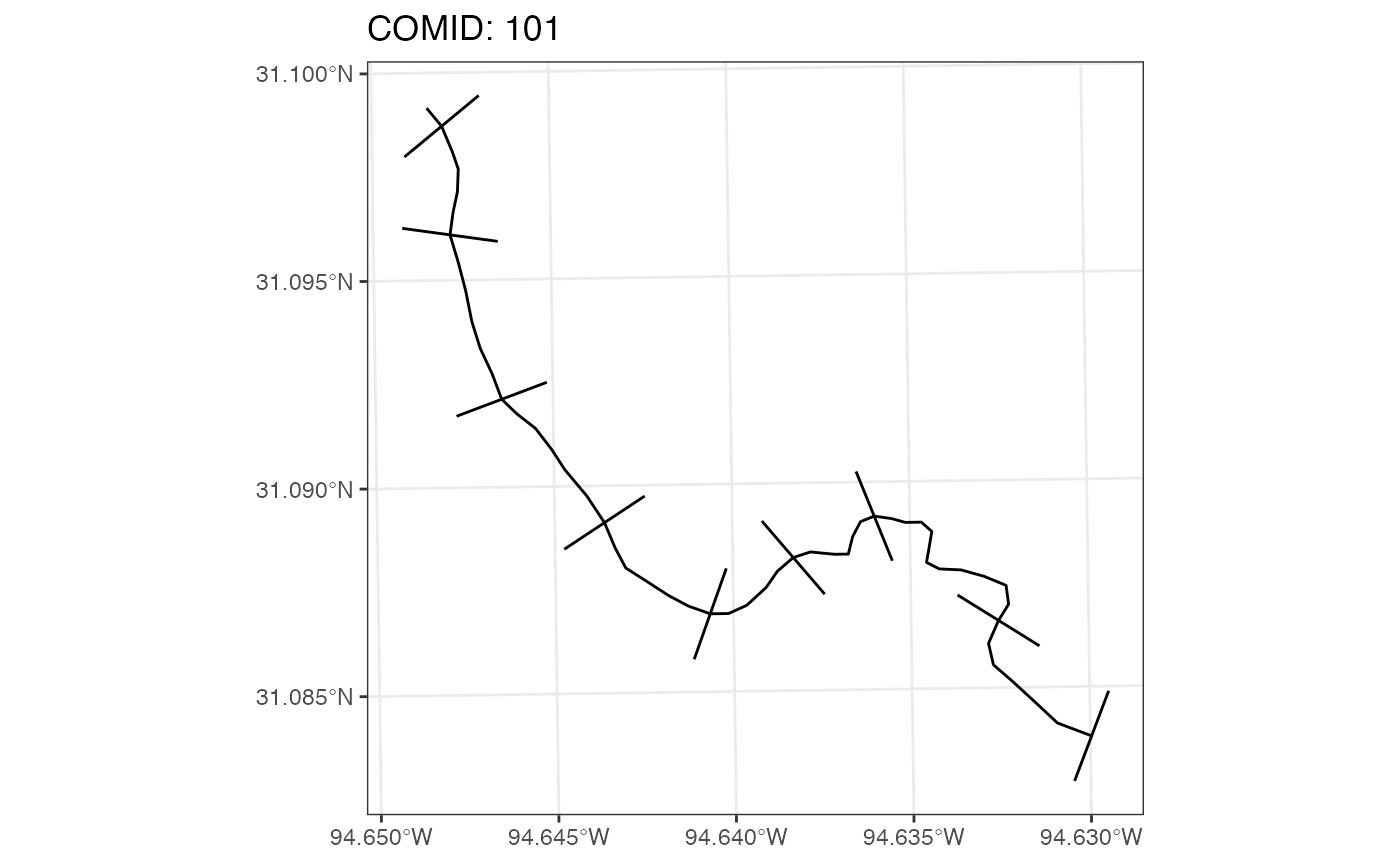
Our algorithm works by generating a set of edges from a single line string, and computing normal vector, that are transformed with a series of afline transformations. To illustrate this lets start with a single flowline:

linestring = filter(network, comid == 101)

Step 1: Explode Linestring into edges:

# sf --> geos object
 line <- as_geos_geometry(linestring)
  
# extract vertices
 vertices <- wk_vertices(line)
  
# Use vertices to reconstruct line segments
  edges <- as_geos_geometry(
    wk_linestring(
      vertices[c(1, rep(seq_along(vertices)[-c(1, length(vertices))], each = 2), length(vertices))],
      feature_id = rep(seq_len(length(vertices) - 1), each = 2)
    )
  )

Step 2: Define Edge Mid and End Point

The next steps are down for each individual edge in the exploded linestring:

# Starting with just the first edge
edge  <-  edges[1]
# Define a width of desired cross section
width <-  linestring$cs_width

# find the midpoint
midpoint <- geos_interpolate_normalized(edge, 0.5)
# find the end point
ep       <- geos_point_end(edge)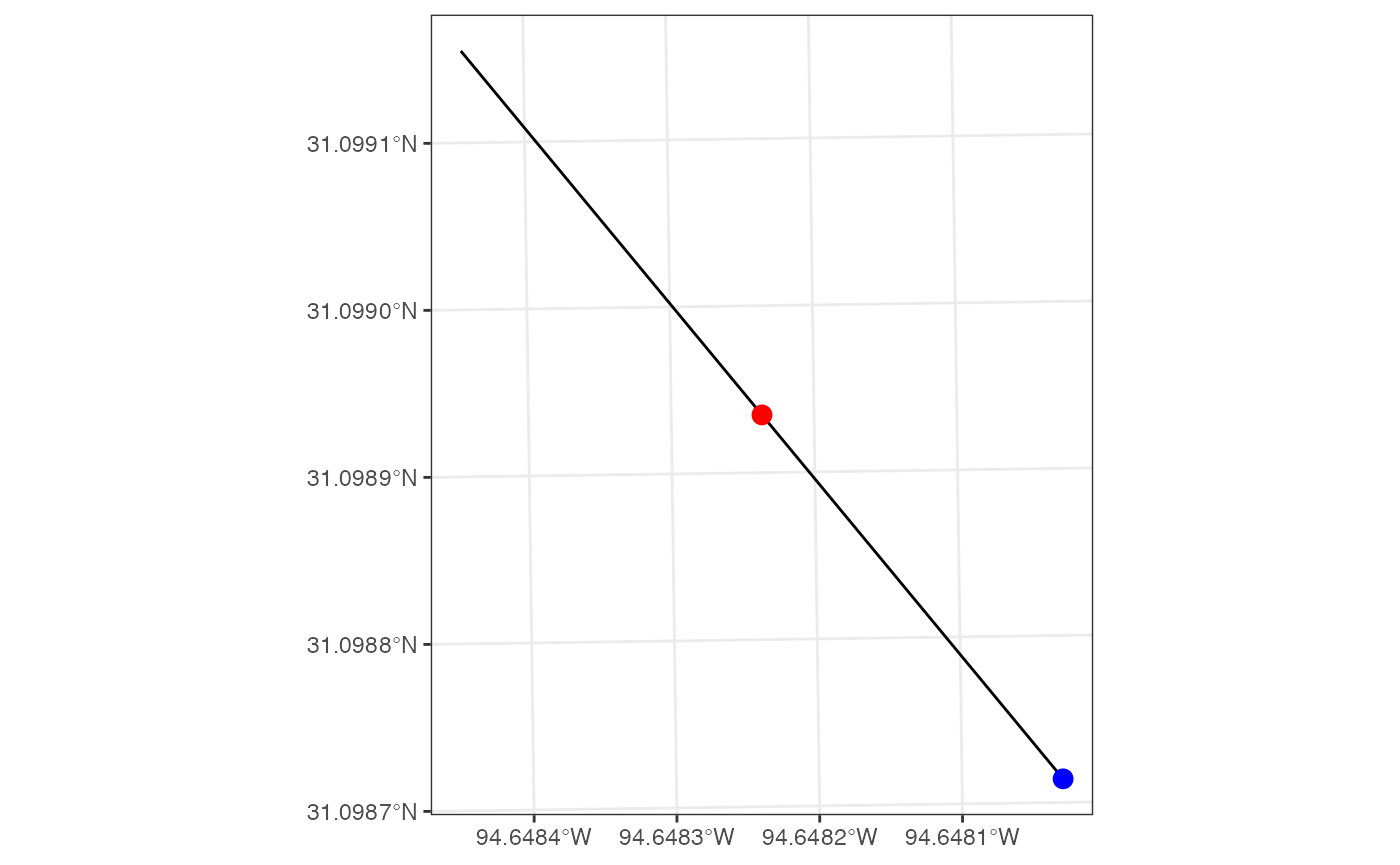

Step 3: Define Cross Section at end Point

To generate a cross section that passes through the end point we need to steps

Define a normal edge

3 transformations to define a normal edge:

affine_translate: define the coordinate offsets in the x, y direction as the negative value of the X and Y coordinate of the edge midpoint
affine_scale: apply an X scale factor of 1/length of the edge, and a Y scale factor of 1/length of the edge
Rotate the new line 90 degrees

normal_edge <- wk_transform(edge, 
                                wk_affine_compose(
            wk_affine_translate(dx = -geos_x(midpoint), dy = -geos_y(midpoint)),
            wk_affine_scale(1 / geos_length(edge), 1 / geos_length(edge)),
            wk_affine_rotate(90)
  ))

Define the cross sections

2 transformations are needed to define a cross section:

affine_scale: apply an X scale factor of the desired width, and a Y scale factor of the desired width
affine_translate: define the coordinate offsets in the x, y direction as the negative value of the X and Y coordinate of the edge end point

Lastly, the CRS of the original line is reassigned.

cs = wk_set_crs(wk_transform(
    normal_edge,
    wk_affine_compose(
      wk_affine_scale(width, width),
      wk_affine_translate(geos_x(ep), geos_y(ep))
    )), wk_crs(line))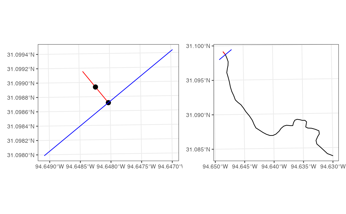

Cut a Full Flowline

Using the above logic, we can write a function that generates a series of cross sections for each edge in the line string:

# Make a function:
cut_transect = function(edge, width){
    
  midpoint <- geos_interpolate_normalized(edge, 0.5)
  ep       <- geos_point_end(edge)
  
  normale_edge <- wk_transform(edge, 
                                  wk_affine_compose(
              wk_affine_translate(dx = -geos_x(midpoint), dy = -geos_y(midpoint)),
              wk_affine_scale(1 / geos_length(edge), 1 / geos_length(edge)),
              wk_affine_rotate(90)))
    
  wk_set_crs(wk_transform(
      normale_edge,
      wk_affine_compose(
        wk_affine_scale(width, width),
        wk_affine_translate(geos_x(ep), geos_y(ep))
      )
    ), wk_crs(edge))
}

system.time({
  all = vec_c(!!!Map(cut_transect, edges, width = linestring$cs_width))
})

##    user  system elapsed 
##   0.049   0.001   0.050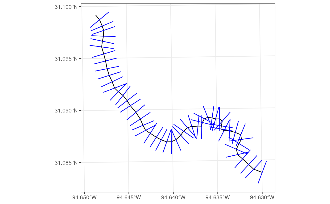

OK that’s pretty good! But there are a few things I don’t like. From here on out we must enforce the following two conditions:

Condition 1: Cross sections should not cross each other
Condition 2: A single cross section should not cross a given reach more then once

Predicates like st_intersect cannot be run at the end without wiping all cross-sections that intersect. So, we need to implement some logic to enforce these:

get_transects = function(edges, line, width){
  
  if(length(width) != length(edges)){
    width = rep(width[1], length(edges))
  }
  
  transects <- geos_empty()
  
  for(i in 1:length(edges)){
    
    tran = cut_transect(edges[i], width[i])
    
    # If a MULTIPOINT, then it crosses more the once
    if(geos_type(geos_intersection(tran, line)) == "point") {
      # Ensure that there are no intersections with previously computed cross sections
        if (!any(geos_intersects(tran, transects))) {
          transects <-  vec_c(transects, tran)
        }
      }
  }

  transects[!geos_is_empty(transects)]

}

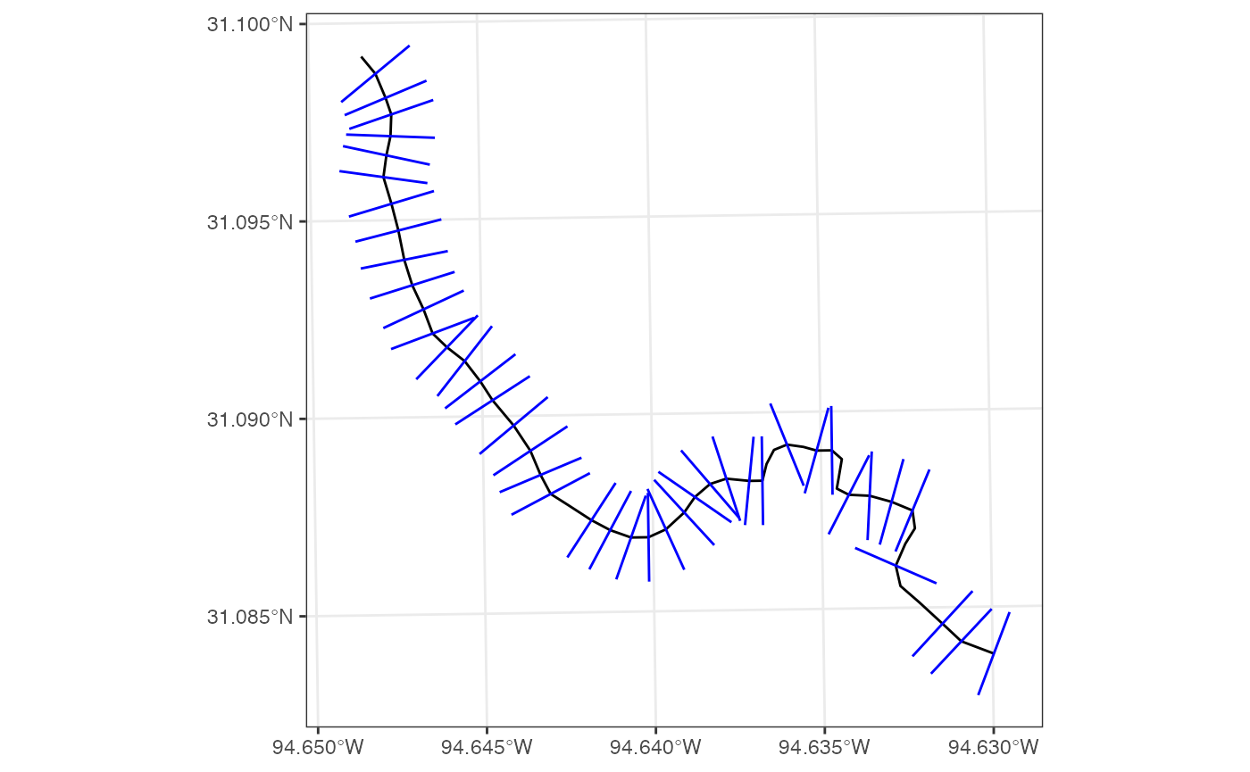
system.time({
 transects =  get_transects(edges, line, width = 250)
})

##    user  system elapsed 
##   0.082   0.001   0.082

Awesome! We gained just a fraction of time while ensuring a set of valid cross sections are generated.

Flow Network

OK, so we have gone from a single edge, to a full flowline. Now - how about a full network! Again, this requires looping over all flowlines. Additionally we add a few new items:

The num argument allows a user to restrict the number of cross sections desired per flowline.
The id argument allows a user to specify the identifier column of the input. If provided these will be assigned as the “hy_id” in the output. If not prescribed, a 1:n() index will be added.
The outputs will also have a 1:n() cs_id describing the ordered set of cross sections where 1 is the most upstream and n is the most downstream.
Lastly, a final pass is made to remove all cross sections that intersect with cross section from a different flowline.

cut_cross_sections = function(net, id = NULL, widths = NULL, num = NULL){
  
  ll = list()
  
  if(length(widths) != nrow(net)){
    widths = rep(widths[1], nrow(net))
  }

  for(j in 1:nrow(net)){
    
   line <- as_geos_geometry(net[j,])
    
   vertices <- wk_vertices(line)
    
    edges <- as_geos_geometry(
      wk_linestring(
        vertices[c(1, rep(seq_along(vertices)[-c(1, length(vertices))], each = 2), length(vertices))],
        feature_id = rep(seq_len(length(vertices) - 1), each = 2)
      )
    )
   
    if(!is.null(num)){
      edges = edges[as.integer(seq.int(1, length(edges), length.out = num))]
    }

    ll[[j]] = get_transects(edges, line, widths[j])
  }

  ids_length = lengths(ll)
  ll = st_as_sf(Reduce(c,ll))
  
  if(!is.null(id)){
    ll$hy_id = rep(net[[id]], times = ids_length)
  } else {
     ll$hy_id = rep(1:nrow(net), times = ids_length)
  }
  
  ll[lengths(st_intersects(ll)) == 1, ] %>% 
    group_by(hy_id) %>% 
    mutate(cs_id = 1:n()) %>% 
    ungroup()
  
}

system.time({
  oo = cut_cross_sections(net = network, 
                          id = "comid", 
                          widths = network$cs_width,
                          num = 10)
})

##    user  system elapsed 
##   6.206   0.057   6.330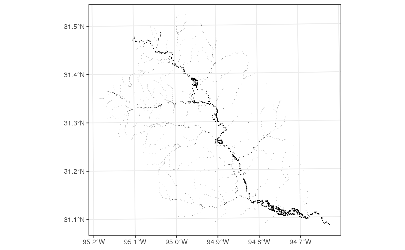

Transects to 3D channel

To turn the extracted transect set into “3D” cross sections, we need to define a set number of points to sample along each line, and then use those to extract an elevation from a DEM. Here, we use a VRT file of the 10m 3DEP elevation data that we produced for the National Map with support from the 3DEP team.

library(terra)
points_per_cs = 35
elev_url = "/vsicurl/https://prd-tnm.s3.amazonaws.com/StagedProducts/Elevation/13/TIFF/USGS_Seamless_DEM_13.vrt"

extract_pt_val = function(rast, pts){ extract(rast, project(vect(pts), crs(rast)))[,2] }

system.time({
  cs_pts = 
      st_set_geometry(oo, st_line_sample(oo, points_per_cs)) %>% 
      st_cast("POINT") %>%
      st_transform(st_crs(rast(elev_url))) %>% 
      mutate(Z   = extract_pt_val(rast(elev_url), .)) %>% 
      group_by(hy_id, cs_id) %>% 
      mutate(pt_id = 1:n()) %>% 
      ungroup()
})

##    user  system elapsed 
##   7.186   0.579  30.226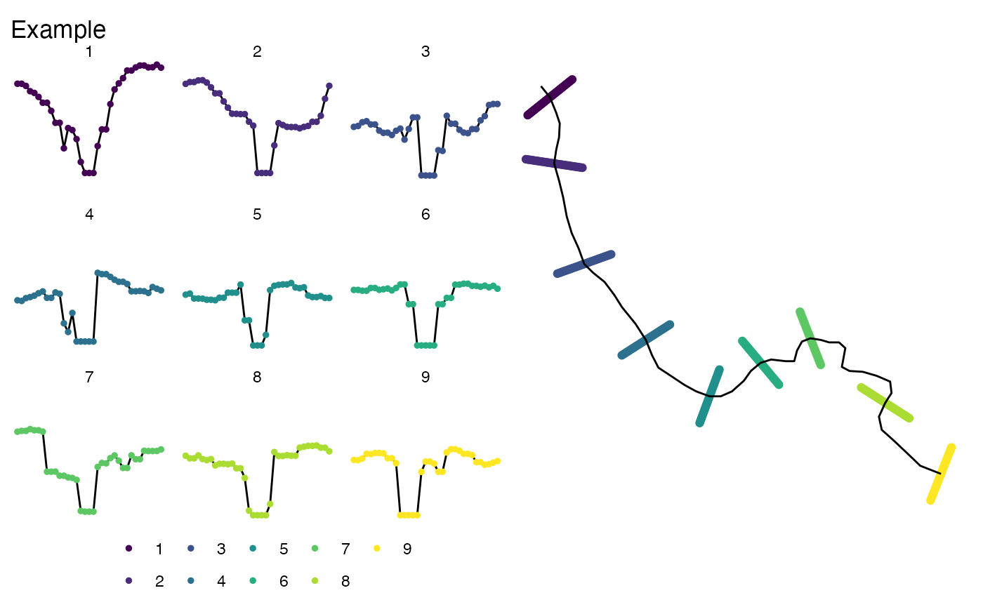

Reach Addressing

A key for hydrologic locations is a linear reference that describes the percentage along a reach a location sits. To reference the center of each cross section, we can use the flowline indexing tools in nhdplusTools:

system.time({
  # Find middle point of each cross section
  tmp = cs_pts %>% 
    group_by(hy_id, cs_id) %>% 
    arrange(pt_id) %>% 
    slice(ceiling(n()/2))  %>% 
    ungroup() %>% 
    st_transform(5070)

  # Add the needed information to our network object, and fine flowline index
  xx = left_join(network, 
                 get_vaa(c("tomeas", "frommeas", 'reachcode'), updated_network = TRUE), 
                 by = c("comid")) %>% 
     get_flowline_index(tmp) %>% 
     mutate(cs_id = tmp$cs_id[id], id = NULL) %>% 
     rename(hy_id = COMID)
  
  # add new information of cs_pts and rearrange columns
  cs_pts = left_join(cs_pts, xx, by = c("hy_id", "cs_id")) %>% 
    select(hy_id, cs_id, pt_id, everything())
})
  
head(cs_pts)

Channel Classifiction

OK so now we have cut cross sections along network, sampled them and extracted depths, and addressed them to the hydrologic network! Now, we want to to assign a classification to each point marking it as “right_bank”, “in_channel” and “left_bank”.

assign_class = function(Z, ratio = 1/5){ 
  
  # The change in elevation across the cross section
  dY = c(diff(Z), 0)
  # devise a threshold for each section based on the prescribed ratio
  thres = ratio * length(Z)
  # Assume the left side is 2* threshold
  la = 2*thres
  # Assume the channel is the left edge plus one part.
  ca = la:(thres + la)
  
  # Assume the channel sits within the middle part + or minus a part
  mid_sec = Z[(2*thres):(length(Z)-2*thres)+1]
  mid = floor(median(which(Z == min(mid_sec) )))
  
  if(mid < 2*thres | mid > 2 * thres){
    mid = min(mid_sec) 
    mid = floor(median(which(mid_sec == mid))) + 2*thres
  }

  lb = which.min(dY[(mid-thres):mid]) + (mid-thres) - 2
  
  rb = which.max(dY[(mid):(mid+thres)])  + mid + 1
  
  class = rep("in_channel", length(Z))
  class[1:lb] = "left_bank"
  class[rb:length(Z)] = "right_bank"
  
  if(length(class) != length(Z) |  dim(table(class)) != 3){
    class = c(rep("left_bank", 2*thres), 
              rep('in_channel', thres), 
              rep("right_bank", 2*thres))
  }
  
  class
}

system.time({
  cs_pts = cs_pts %>% 
    group_by(hy_id, cs_id) %>%
    mutate(class = assign_class(Z, ratio = 1/flood_plain_sections)) %>% 
    ungroup()
})

mapview::mapview(network)

Channel bottom alignment and bank smoothing

Lastly, for a successful routing implementation, we need to ensure that the bottom of each cross section is lower then or equal to that one upstream. Here we will traverse down the network making sure this condition is met, and, in cases where it isn’t, we will lower the in channel portion of the cross section to make it so:

Mike Johnson