Goals

Already you should have R and RStudio on your machine. You should also have a Github account and should be comfortable creating a new repository and connecting in to a new R Project in your ~/github folder. Building on these, this lab has a few key learning objectives.

It will ensure you are comfortable with the tools of reproducible science including:
- RStudio (for developing),
- Rmarkdown (for authoring)
- Github (for version control and publishing)
It will provide a central repository for your work throughout the quarter
It will become an artifact you can take with you to showcase your skills to future employers.

By the end of this activity you will have:

Constructed a simple website with basic information
Hosted it your personal Github for the world to see
Been exposed to markdown, YMAL, CSS, HTML and website construction
Practiced Forking and contributing to another repository.

All said, the more time you put into refining, personalizing and developing this site through the quarter, the more it will benefit you in the long run, both in this class and beyond!

Okay, let’s get started.

Jargon

As with any field, web development (or web communication!) has its own lingo and toolsets. Here is a brief summary of the unfamiliar terms you will see in this activity:

URL: URL stands for Uniform Resource Locator and is a reference to a web resource specifying its location on a computer network and a mechanism for retrieving it. Think of it as a web address.
HTML: HTML stands for Hyper Text Markup Language. HTML is the standard markup language for Web pages. Remember that we knit our markdown (Rmd) files to HTML.
CSS: CSS stands for Cascading Style Sheets. CSS describes how HTML elements are displayed. Should a header (#) be blue? Green? Orange? CSS saves a lot of work because it can control the layout of multiple web pages at once.
YML (or YAML): YAML (stands for “YAML Ain’t Markup Language”) is a human-readable data-serialization language. It is commonly used to configure “global” information. In Rmarkdown files, it describes how the file should knit.

Website Hosting

GitHub Pages

GitHub Pages is a static site hosting service that takes HTML, CSS, and JavaScript files straight from a repository and publishes them as a website. GitHub Pages is available for public repositories.

There are three types of GitHub Pages sites: project, user, and organization.

We are not interested is organization sites, and will focus on the details of user and project sites.

In this lab, we will be building your user site, and in future labs, you might build a project site.

user sites are connected to a GitHub account (not a project/repository). To publish a user site, you must create a repository named <user>.github.io. Active user sites are available at http(s)://<username>.github.io.
project sites are connected to a single project (repository). The source files for a project site are stored in the same repository as their project. Active project sites are available at URLs following the pattern: http(s)://<username>.github.io/<repository>.

Why are Github Pages cool? Well they are free. They are secure. And like the versioned code, all you need to do to modify a sites is edit, commit, and push your changes.

Set up

These first steps will be used in every lab, and we outline them in detail here:

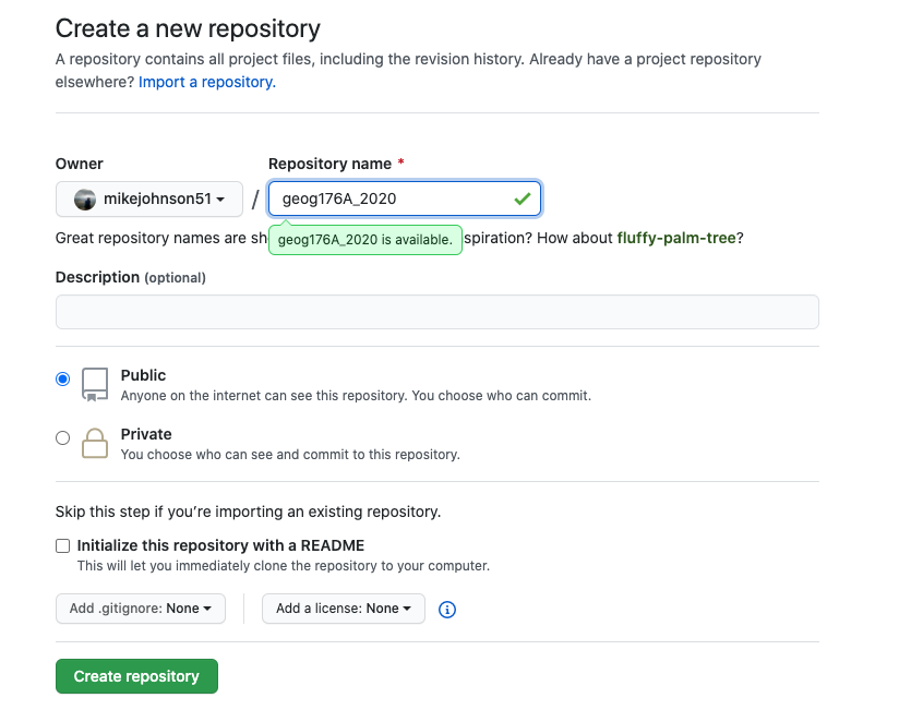
Create a new repository on your Github account named: <username>.github.io. The following image shows the process but the repositoty name should be your username!!

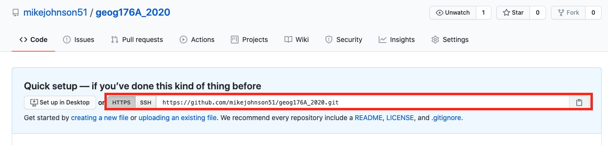
Once created, copy the repositories URL

Launch RStudio
Create a new version controlled project using the Github URL
- File –> New Project –> Version Control –> Git
- Enter the Github URL, keep the default name, and create the project as a sub directory of your ~/github folder

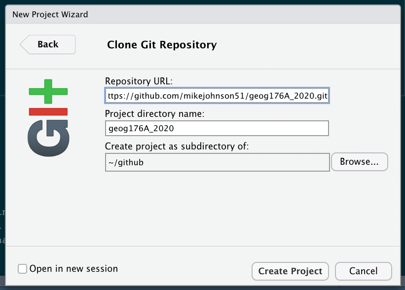
Create the project!

Building your content

Initiating the needed files:

To build a website, we need to initialize a couple empty files in our repository. We will do this using the terminal! Go ahead create three new files in our <username>.github.io project:

"_site.yml" (the underscore is needed!)
“index.rmd”
“geog13.rmd”

_site.yml tells your website how to assemble itself

index.Rmd is the main Rmd file

geog13.Rmd provides a home page for this course

Last, make a new directory called img

Your resulting project should match this structure:

fs::dir_tree("first-webpage")

## first-webpage
## ├── _site.yml
## ├── geog13.rmd
## ├── img
## └── index.rmd

Now open all of these files in RStudio.

Filling in our information

_site.yml

We will start by filling out the yml file. yml files provide a road-map telling R how to assemble a website. We use a yml file to specify how our website looks, just as we use yml in the header of an Rmarkdown file to define how our document renders. yml files are super sensitive to tabbing so make sure your spacing is correct if problems arise.

We want to tell our site 4 things:

What is the name of the site
Where should the HTML files knit to? (output_dir)
That we want a nav-bar and
What should be in the nav-bar

We can do this by filling in the appropriate yml metadata (make name and title more meaningful to you…):

name: "first-website"
output_dir: "."
navbar:
  title: "My Beautiful Website"
  left:
    - text: "Home"
      href: index.html
    - text: "GIS Work"
      href: geog13.html

Think about the relationship between the href elements and the output directory! How does this align with what we learned about file paths?

The navbar

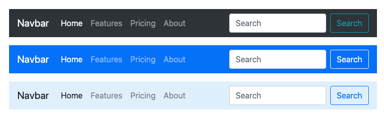
navbar references Bootstrap’s powerful, responsive navigation header. The “navbar” includes support for branding, navigation, and more. Bootstrap is one of the world’s most popular front-end open source toolkits and is integrated (in a limited way, with knitr/rmarkdown). We not only use Bootstrap elements here, but will apply Bootstrap themes, later on. An example of a “navbar” can be seen below:

In our navbar we state there should be a title - “My Beautiful Website” - and on the left side of the navbar, two text strings, one that says “Home” and one that says “GIS Work”. If someone clicks on “Home” it will redirect (href = hyperlink reference) them to a file called “index.html”. Equally, if they click on “GIS Work” they will be redirected to an HTML file called, “geog13.html”.

navbars are really common. See an example of a navbar with icons and themes on ‘ResearchGates’ main page:

At this point, we do not have an index.html or geog13.html file to point to, so, lets make those:

index.html

index.html is the most common name for the default page shown on a website. If you publish a website, and a server looks for the web address, the information rendered is likely stored in the index.html file. Therefore it is critical you have a file named index.html if you are going to host your own site.

We will use your websites landing page as an “about me” section to introduce yourself to our class and more broadly to the internet. Take some time to write a concise and clear paragraph introducing yourself, describing what you enjoy, and what you aim to do (within a professional context). Feel free to add hyperlinks to relevant accounts or other web pages using the Rmarkdown syntax.

A nice example of an ‘about me’ can be found on James Clears website:

If we wanted to replicate this in markdown we would need something like the following in our index.Rmd:

---
title: "About Me"
---
  
<center>
# Hi, I'm Mike Johnson.
</center>
  
[Lorem ipsum](https://www.lipsum.com/) dolor sit amet, consectetur adipiscing elit, sed do eiusmod tempor incididunt ut labore et dolore magna aliqua. Ut enim ad minim veniam, quis nostrud exercitation ullamco laboris nisi ut aliquip ex ea commodo consequat. Duis aute irure dolor in reprehenderit in voluptate velit esse cillum dolore eu fugiat nulla pariatur. Excepteur sint occaecat cupidatat non proident, sunt in culpa qui officia deserunt mollit anim id est laborum.

Which would render as:

Hi, I’m Mike Johnson.

Lorem ipsum dolor sit amet, consectetur adipiscing elit, sed do eiusmod tempor incididunt ut labore et dolore magna aliqua. Ut enim ad minim veniam, quis nostrud exercitation ullamco laboris nisi ut aliquip ex ea commodo consequat. Duis aute irure dolor in reprehenderit in voluptate velit esse cillum dolore eu fugiat nulla pariatur. Excepteur sint occaecat cupidatat non proident, sunt in culpa qui officia deserunt mollit anim id est laborum.

Your job is to make this paragraph meaningful to you, and to add a image of yourself (or something relevant to you) using Rmarkdown or HTML syntax. The image should be saved in the appropriate img folder following the basic structure of an solid project.

The image can go above, below, or beside your text. After all, this is your website!

Make sure to knit regularly to see how your changes are taking effect.

geog13.html

We will treat geog13.Rmd as a “projects” page for this class. Here we will describe and link to the projects and activities we do through the quarter. Below is an example:

---
title: "Projects"
---

In the summer of 2021 I took a class GIS course based in R. I worte some code, and did some cool data science. Here is a collection of links! 

## [Building a project website]()

- In this assignment we built a static users site with Github Pages 
- Includes a github repo for access to all the code.
- Look at how high quality my work is!

Your job is to make this text meaningful to you, and to add the appropriate URL to the header. You must also describe what you learned in this activity in 3-5 bullet points. Do this in a way that is directed at showing an audience what you know, not as an exercise to satisfy me.

Build your site

The minimum requirement for an R Markdown website is an index.Rmd file and a _site.yml file. We have each of these! Now you can run render_site() in the console.

rmarkdown::render_site()

When you do this, the following occurs:

All *.Rmd and *.md files in the root directory are rendered into HTML.
- Markdown files beginning with **_** are not rendered (a convention to designate files that are to be included by top level Rmd documents as child documents).
The generated HTML files and any supporting files (such as CSS and JavaScript) are copied into an output directory (_site/ by default).
- However! If you look at the yml file we created, we OVERRODE this default by defining the output_dir as “.” -or- the root project directory.

Now if everything has gone according to plan, by running the code you should get a bunch of unintelligible output followed by the message:

Output created: index.html

If so, 🎉 congrats 🎉, if not, double check all the stuff above and make sure you are in the right directory (try pwd in the terminal).

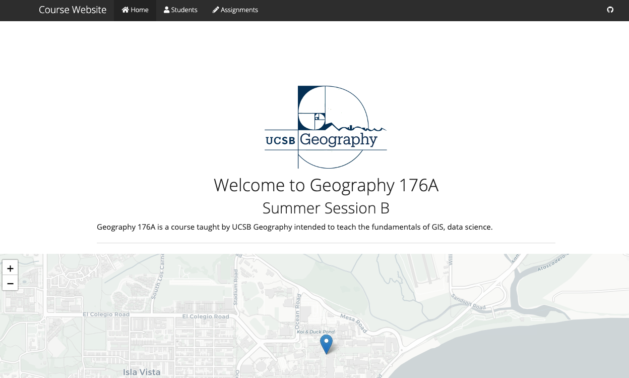
Go ahead and open index.html in a browser (right click on the file in the RStudio files tab) to see your website!

That is pretty awesome but is notably a bit ugly… lets make it better!

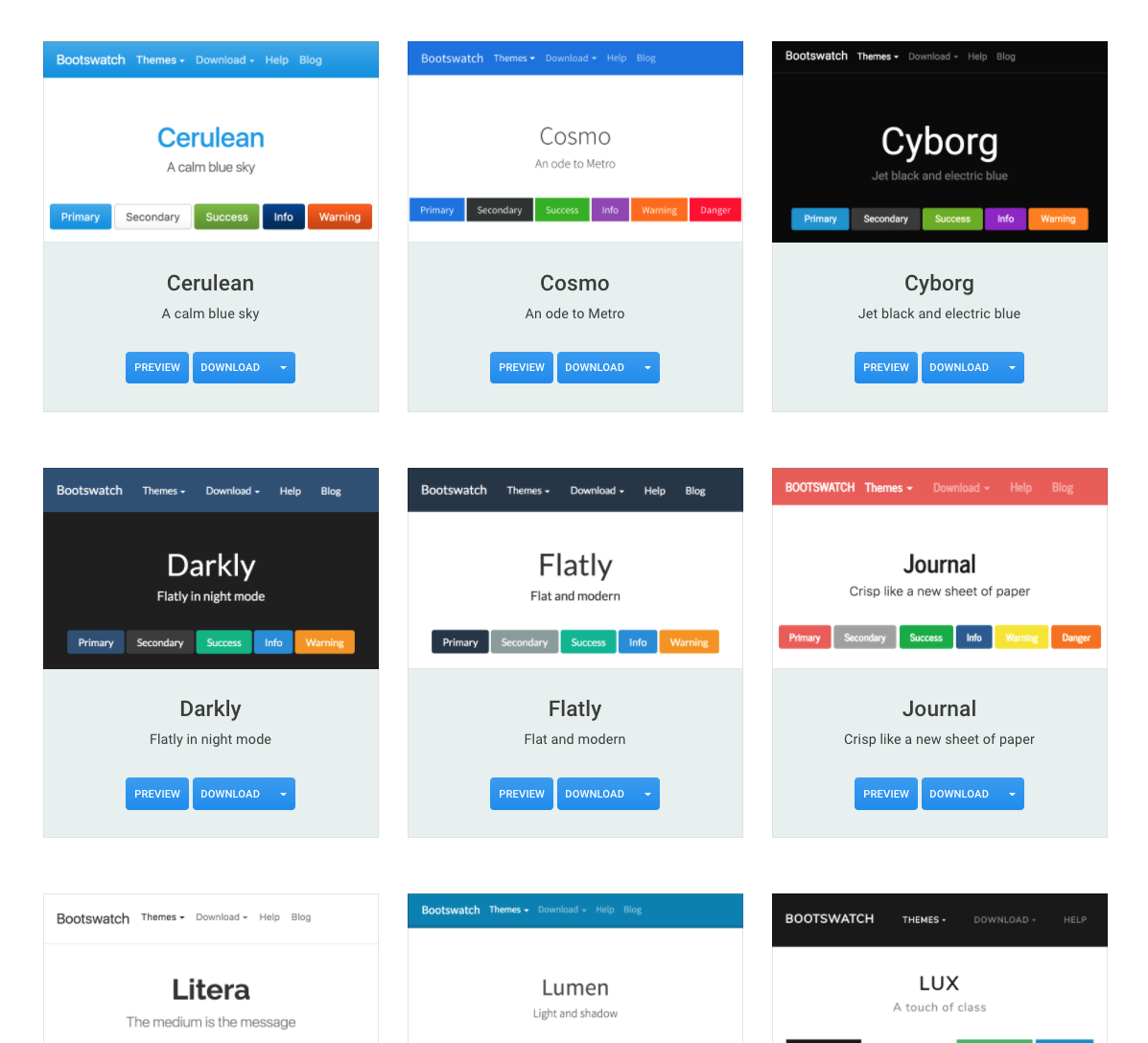
Website theme

Remember our friend Bootstap? Well, the html_document engine uses the Bootswatch theme library to support different styles of documents. Bootswatch simply provides free themes for Bootstrap. Check out the above link to see which theme you like, or the image below:

You can also check which themes are valid for the html_document engine:

## Note the 3 :::
rmarkdown:::themes()

##  [1] "default"   "cerulean"  "journal"  
##  [4] "flatly"    "darkly"    "readable" 
##  [7] "spacelab"  "united"    "cosmo"    
## [10] "lumen"     "paper"     "sandstone"
## [13] "simplex"   "yeti"

To control the output styles of an HTML document in R Markdown, we must specify the output format (html_document) in the YAML metadata. Only by doing this can we specify the theme we want to use. For an example, see our modified _site.yml below, again remembering that tabbing is sensitive:

name: "first-website"
output_dir: "."
navbar:
  title: "My Beautiful Website"
  left:
    - text: "Home"
      href: index.html
    - text: "GIS Work"
      href: geog13.html
output:
  html_document:
    theme: darkly

Test a few different themes (change the theme and run rmarkdown::render_site()) to find the one you like!

Icons

Font Awesome is a font and icon toolkit based on CSS. It was made for use with Bootstrap, and later was incorporated into the BootstrapCDN. Font Awesome provides scalable vector icons (SVGs) that can be customized (size, color, drop shadow, etc).

The complete set of icons can be see here. Many of them only come with the paid “pro” version, but there are still many that are free to!

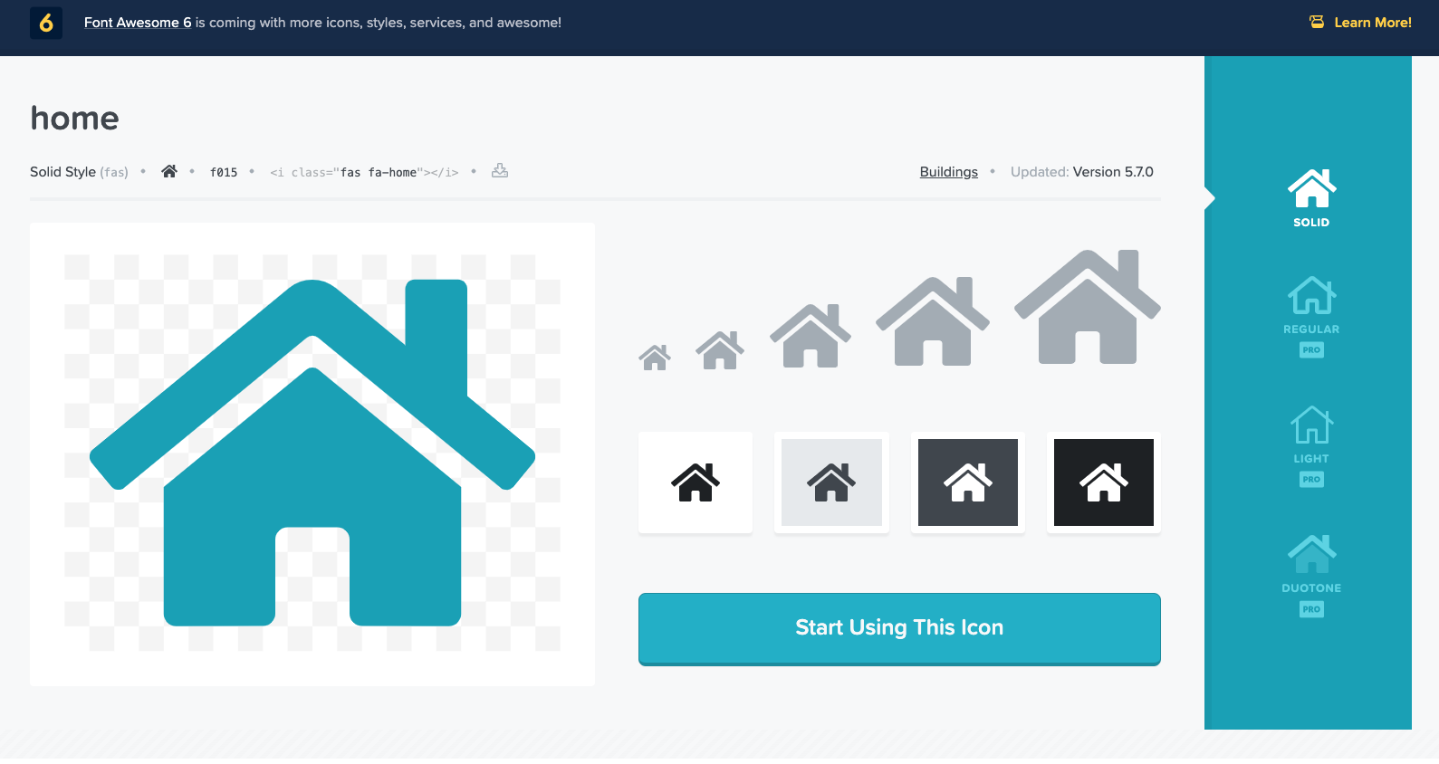
In the above image, we are looking at the “home” icon on fontawesome.com, with the link. Here we see the “home” icon is identified as “fas-home” where the “fas” is “Font Awesome Solid” and “home” is name. There are many ways that we can use these icons, lets take a look at a few of them:

In the navbar

Icons can be added to the navbar as either the primary, or sub, element, of a link. Below we see a code chunk from our yml file that places the fa-home icon next to the hyperlinked text “Home”, and the fa-github icon serving as the hyperlinked object directly. Notice also that the github logo has been placed on the right side of the navbar per the yml.

  left:
    - text: "Home"
      icon: fa-home
      href: index.html
  right:
    - icon: fa-github
      href: https://github.com/mikejohnson51/geog13

The result of this would be something similar to:

Currently, direct support for icons in rmarkdown is limited to FA-4 (see github issue here). I will update this when/if it changes. Until then, valid FA-4 icon names can be found here

FA as HTML

Icons can also be called directly by HTML. For example, if we wanted to place the home icon in our text, we could simply add:

<i class="fa fa-home"></i>

To get an icon like:

We could change the size of the icon by growing it by some amount “X”. For example to make our icon 3 times bigger:

<i class="fa fa-home fa-5x"></i>

To get an icon like:

We can also use the HTML Tag to dictate the color under the objects style. So if we wanted to make it red we could add code like:

<i class="fa fa-home fa-5x" style="color:red;"></i>

To get an icon like:

Though the `icons` package

Granted using HTML to add & control these icons is not “hard” but it is tedious and difficult to remember the syntax. One of the great things about R and the R community, is that developers create packages to help us overcome typical hurdles. One of these is the icons package. icons is not on CRAN, so we must download it from Github using the remotes package:

NOTE: One of the great things about open source code is that it is often improving. These regular improvements can introduce “breaking” changes at time. It is typically avoid, but other times impossible. For this lab, if the new icons package (which supersedes the icon) package has a few breaking changes as noted here

Icons are no longer included directly in the package, and will require downloading before use. Use the download_*() functions to download an icon library you want to use.
The short names (fa, ii, etc.) have been replaced with longer, more informative names (fontawesome, ionicons, etc.).
Animations of icons is no longer supported (this functionality will be made possible in a new package specific to CSS animations).

The following directions have been updates to match this new package syntax:

# install.packages("remotes") ## if not installed
remotes::install_github("ropenscilabs/icon")
# download the font awesome library
download_fontawesome()

library(icons)
# Call by fa name
fontawesome("rocket")

#is the same as calling by list element:
fontawesome$solid$rocket

# Can change the size by updating the icon "style"
icon_style(fontawesome("rocket"), scale = 2)

# And the color!
icon_style(fontawesome("rocket"), scale = 5, fill = "yellow")

And since this is is a class that hopefully gets you loving R and Spatial data, lets add a series of icons in line:

`r icon_style(fontawesome("globe"), scale = 5, fill = "green")` 
`r icon_style(fontawesome("plus"), scale = 2, fill = "black")` 
`r icon_style(fontawesome("r-project"), scale = 5, fill = "blue")`   
`r icon_style(fontawesome("equals"), scale = 2, fill = "black")` 
`r icon_style(fontawesome("heart"), scale = 5, fill = "red")`

Take some time to personalize your yml, index, and geog13 files with a few icons.

Commit/Push

You now have an awesome set of documents ready to share, but since they are only on your machine, they cannot be made into a website. To do that we need to get our files to Github, and, tell Github to host it as a site! Now that you have all your code ready to publish, go ahead and stage/commit/push your work to GitHub!

Activate the Webpage

From your repo (once your push has cleared):

Navigate to Settings –> Pages
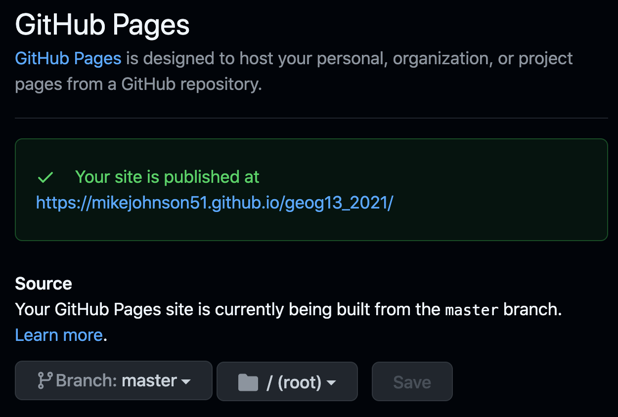
Change the source to master branch and the folder to root.
At the top, a URL will appear telling you your pages are published. Copy that URL.

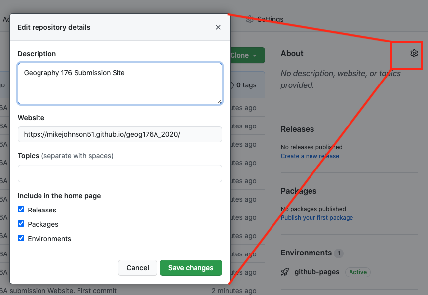
Return to the repositories main page and click the Settings icon () next to “About”
Paste your URL under website, and add a brief description (see below)

Note: github has to build stuff on its end so it may take a minute or so for changes to render to show up. Just keep refreshing the page and it will go faster.

🎉 Congrats 🎉 you have created a personal website and hosted it online.

Add a CV

Ok, now it’s on you!

Practice what you’ve learned by creating a brief CV.

Create a new Rmarkdown file
The title should be your name, and you should include headings for (at least) education and experience.
Each of the sections should include a bulleted list of things you find important (Highlight the year in bold)
Add the CV/Resume as a link in your websites navbar and ensure it is referenced correctly
Render your site
Push the updates to GitHub

Submitting your assignment.

I have created a repository here for our class. Notice, it is identical to the site you just built with some minor modifications.

To submit your assignment, you must do the following:

Fork the above repo (click)
Make a local copy as an RProject in your ~/github directory
Update the index.Rmd with an H4 heading (####) including:
- A colored icon unique to you
- Your name in bold
- The text “repo” linked to your repo
- The text “webpage” linked to your website
Under that, as a list add:
- Your year and major (with the “user” icon )
- An area of research you enjoy (with the “university” icon ).
- The lat long of where you are taking this class form: (with the “map-marker” icon ).
- An example of what we want would look like this:

Mike Johnson repo — webpage

Instructor
Water Resources
34.41, -119.84

Knit (button or CMD+SHIFT+K) roster.Rmd with your additions and make sure it looks right,
Commit your changes to your local copy,
Push the changes to your online repo,
Submit a pull request to have your modifications merged with my master branch doing the following:

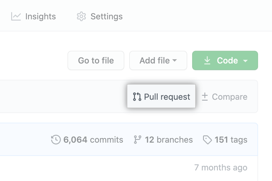
On GitHub, navigate to the main page of your version of the geog13_2021 repository.
Above the list of files, click Pull request.

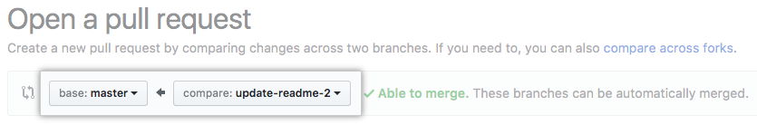
Use the base branch dropdown menu to select the branch you’d like to merge your changes into (my master), then use the compare branch drop-down menu to choose the topic branch you made your changes in (your master).

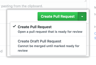
Type a title and description for your pull request.

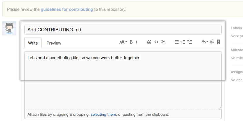
Create a pull request that is ready for review, by clicking “Create Pull Request”.

When you do this, I will merge your changes into the master site. In addition, submit your webpage URL to the appropriate Gauchospace dropbox.

Lab 1

Publishing an RMarkdown Website on Github

Mike Johnson - Lab 01

Goals

Jargon

Website Hosting

GitHub Pages

Set up

Building your content

Initiating the needed files:

Filling in our information

_site.yml

The navbar

index.html

geog13.html

Build your site

Website theme

Icons

In the navbar

FA as HTML

Though the `icons` package

Commit/Push

Activate the Webpage

Add a CV

Submitting your assignment.

Mike Johnson repo — webpage

Rubric

Lab 1

Publishing an RMarkdown Website on Github

Mike Johnson - Lab 01

Goals

Jargon

Website Hosting

GitHub Pages

Set up

Building your content

Initiating the needed files:

Filling in our information

_site.yml

The navbar

index.html

geog13.html

Build your site

Website theme

Icons

In the navbar

FA as HTML

Though the icons package

Commit/Push

Activate the Webpage

Add a CV

Submitting your assignment.

Mike Johnson repo — webpage

Rubric

Though the `icons` package