Geography 13

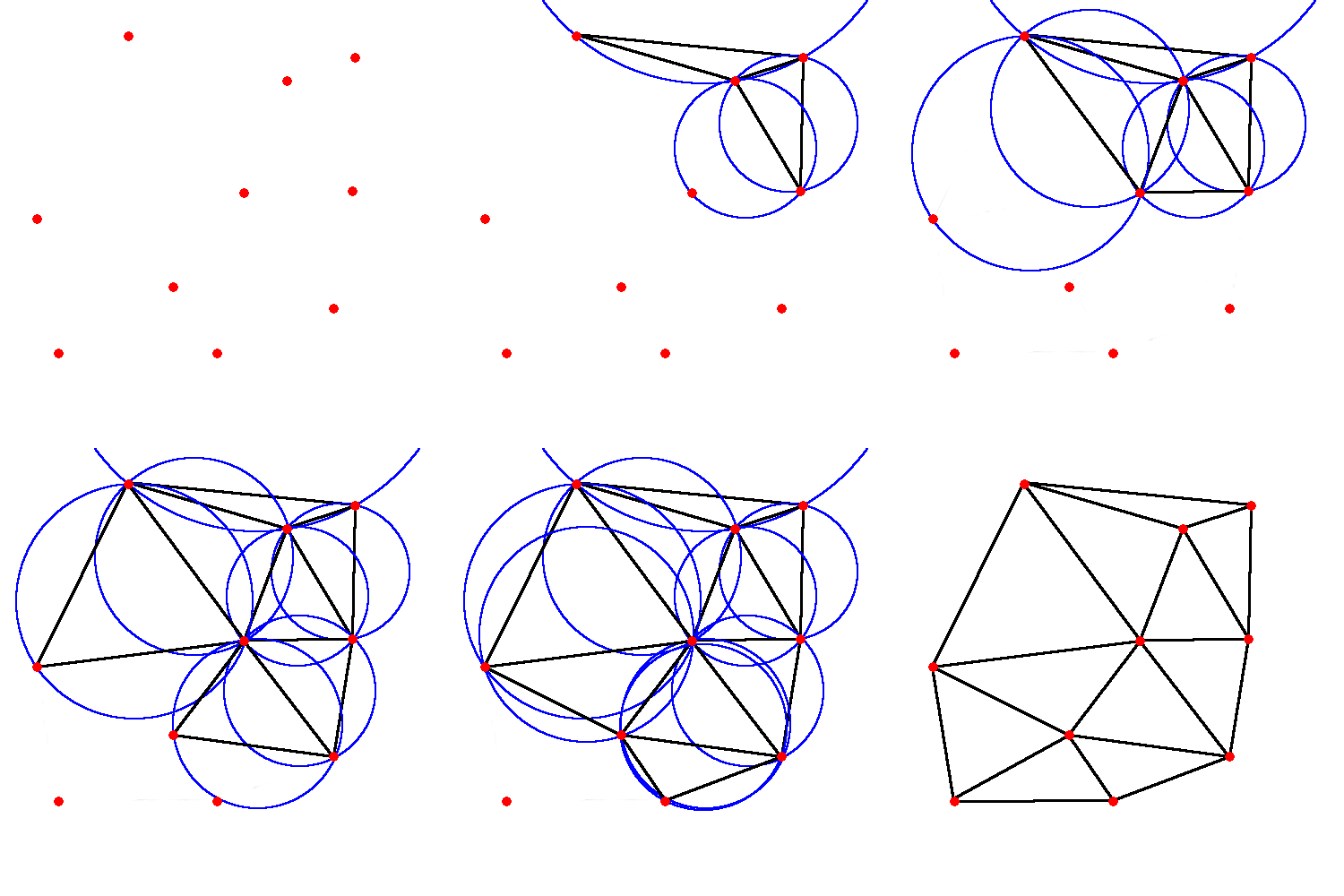
class: center, middle, inverse, title-slide

# Geography 13
## Lecture 16: Interactive Mapping
### Mike Johnson

---

# Yesterday

- Talked about the object/field view of spatial data

- Looked at object coverages

- Specifically grid, hexagon, triangulation, and voronoi polygon ...

--
  - **grid** = standard, raster view
  - **hexagon** = more efficient and better curvature (more complex matrix algebra)
  - **Voronoi** = polygons presenting the area closest to a point
  - **Triangulation** = all points treated as coverage vertices

---

# Coding is hard

- Just this week I have made mistakes with the name `id` in the PIP function

- yesterday in lab, we needed a hexagon rather then square grid to implement a generalized voronoi

- The advantages:
--

- we solve a problem once and wrap it as a function for latter re-use...

- We are closer to the data...

- have flexibility to work beyond existing toolboxes ...

- access to both data and geographic data science methods (attributes and geometry are equal players)

---

.pull-left[

## Voronoi Polygons

![](lec-img/15-Voronoi_growth_euclidean.gif)
]

.pull-right[

## Delaunay Triangles

![](lec-img/15-Delaunay_triangles.gif)
]
---

# Leaflet

- Leaflet is a very popular, open-source, java-script library for interactive maps

- Used by the New York Times, Washington Post, and GitHub, OpenStreetMap, Mapbox and CartoDB

---

# Features

- Interactive panning/ zooming

- Like ggplot, maps are built though combinations of map tiles, markers, polygons, lines, popups

---

# Map Tiles

A tiled web map, or slippy map, is a map displayed in a browser by seamlessly joining dozens of individually streamed over the Internet.

- Most tiled web maps follow certain Google Maps conventions:

--
  
  - Tiles are 256x256 pixels
  
--
  
  - At the outer most zoom level, 0, the entire world can be rendered in a single map tile.
  
--

- Each zoom level _doubles_ in both dimensions, so a single tile is replaced by 4 tiles when zooming in. 
  
--

- This means that about 22 zoom levels are sufficient for most practical purposes.
 
--

- The Web Mercator projection (EPSG:3857) is used, with latitude limits of around 85 (-85) degrees.
 
 
---
 
The OpenStreetMap **standard**, known as Slippy Map  or XYZ, follows these and adds more:

- An X and Y numbering scheme

--
  
  - PNG images for tiles

--
  
  - Images are served through a Web server, with a URL like http://.../Z/X/Y.png, where Z is the zoom level, and X and Y identify the tile.

---

# Zoom Levels

- Zoom Levels define the scale of the map.

- At zoom level 0, an entire mercator projection of the earth is contained in one 256px by 256px tile:

---

---

# Projection Distorition

---

# Zoom Factor 1

At increasing zoom levels the number of tiles increases by a factor of four and the spatial resolution (ground meters per pixel) of each tile roughly doubles.

---

At any given zoom level, a specific tile can be identified by cartesian coordinates with 0,0 starting in the top left of the map.

---

# Request Format

Tiles are requested from a standard URL format:

`url/Z/X/Y.png`

For UCSB the URL:  https://a.tile.openstreetmap.org/18/43803/104352.png

Would return the following image:

---

The horizontal distance represented by each 256x256 pixel tile, measured along the parallel at a given latitude, is given by:

`$$Stile = C ∙ cos(latitude) / 2^{zoomlevel}$$`
--

****

where `$C$` is the equatorial circumference of the Earth for the reference geoid

`$$OSM =  2pi * 6,378,137.00$$`
--

****

As tiles are 256-pixels wide, the horizontal distance represented by one pixel is:

`$$Spixel = Stile / 256$$`

****

For UCSB the URL:  https://a.tile.openstreetmap.org/18/43803/104352.png

```r
C = 2*pi*6378137.00
(Stile = C * cos(34.4140 *pi/180) / 2^18)
```

```
[1] 126.1173
```

```r
Stile / 256
```

```
[1] 0.4926459
```

---

# User Zooming

---
class: center, middle

### Interactive Document [here](https://mikejohnson51.github.io/leaflet-intro/)

You can also fork the [repo](https://github.com/mikejohnson51/leaflet-intro), clone it in RStudio, and use interactively...

All data is in the `data` folder

The examples are in the `index.Rmd` file

---

# Summary

- Interactivity is a great way to highlight and represent data

- Leaflet maps are rendered as HTML objects that can be placed directly in your Rmd files

- You can add markers and shapes to basemaps and annotate them with color ramps, popups and labels

- There is a ton of ability to control and refine your maps in R

- These are extended by libraries like leafem, leafpop and mapview

---

# Daily Assignment

- In an Rmd file, make a leaflet map of data of your choosing

- You are free to double dip on the extra credit in lab 4

- Add at least one feature (table, inset map, custom marker/popup)

- Render it as HTML

- Submit the HTML file to the gauchospace dropbox