Welcome to climateR

Usful Packages for climate data

library(AOI)
library(terra)
library(climateR)
library(tidyterra)
library(ggplot2)
library(tidyr)
library(sf)

climateR examples

The climateR package is supplemented by the AOI framework established in the AOI R package.

To get a climate product, an area of interest must be defined:

AOI = aoi_get(state = "NC")
plot(AOI$geometry)

Here we are loading a polygon for the state of North Carolina More examples of constructing AOI calls can be found here.

With an AOI, we can construct a call to a dataset for a parameter(s) and date(s) of choice. Here we are querying the PRISM dataset for maximum and minimum temperature on October 29, 2018:

system.time({
 p = getPRISM(AOI, 
              varname = c('tmax','tmin'), 
              startDate = "2018-10-29")
})
#>    user  system elapsed 
#>   1.043   0.149   3.232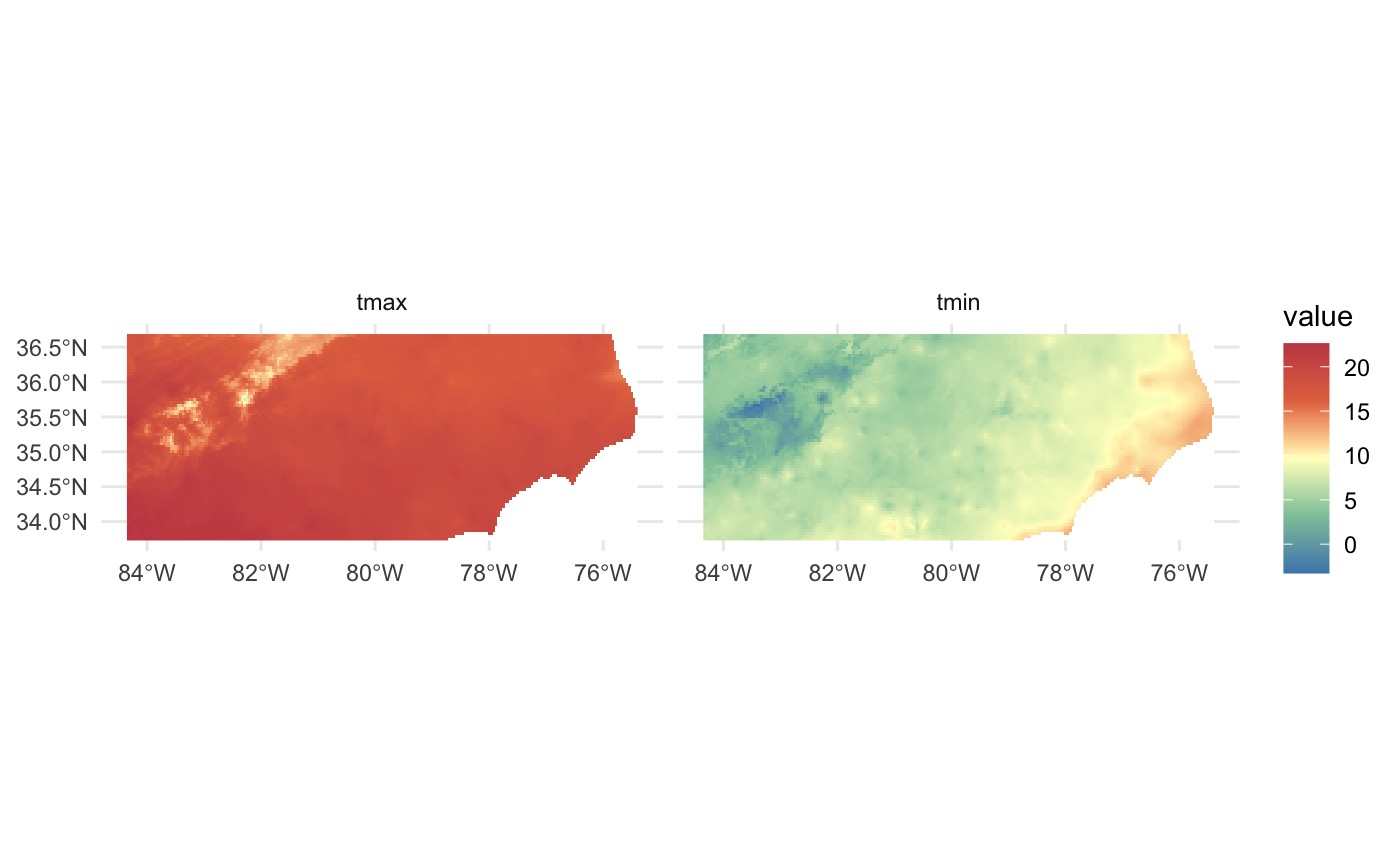

Data from known bounding coordinates

climateR offers support for sf, sfc, and bbox objects. Here we are requesting wind velocity data for the four corners region of the USA by bounding coordinates.

AOI = st_as_sfc(st_bbox(c(xmin = -112, xmax = -105, ymax = 39, ymin = 34), crs = 4326))

g = getGridMET(st_as_sf(AOI), 
               varname = "vs",
               startDate = "2018-09-01")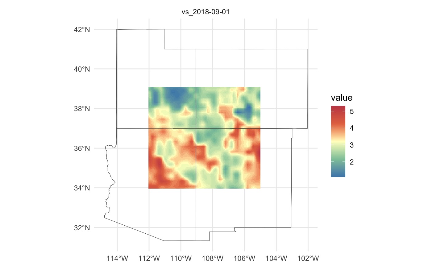

Data through time …

In addition to multiple variables we can request variables through time, here let’s look at the gridMET rainfall for the Gulf Coast during Hurricane Harvey:

harvey = getGridMET(aoi_get(state = c("TX", "FL")), 
                  varname = "pr", 
                  startDate = "2017-08-20", 
                  endDate = "2017-08-31")

ggplot() +
  geom_spatraster(data = harvey$precipitation_amount) +
  facet_wrap(~lyr) +
  scale_fill_whitebox_c(
    palette = "muted",
    na.value = "white") + 
  theme_minimal()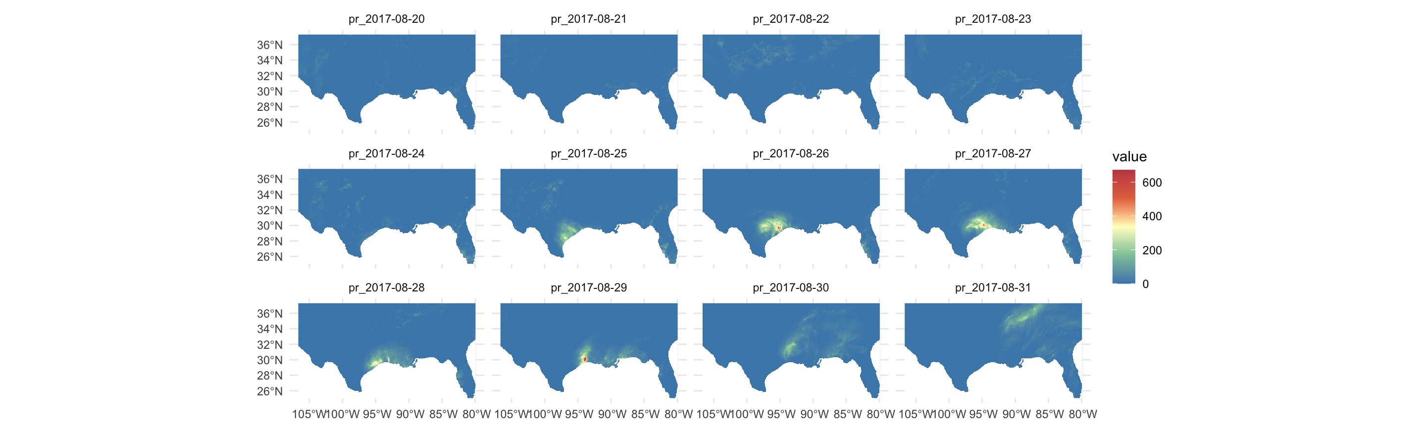

Climate Projections

Some sources are downscaled Global Climate Models (GCMs). These allow you to query forecasted ensemble members from different models and/or climate scenarios. One example is from the MACA dataset:

system.time({
m = getMACA(AOI = aoi_get(state = "FL"), 
            model = "CCSM4", 
            varname = 'pr', 
            scenario = c('rcp45', 'rcp85'), 
            startDate = "2080-06-29", endDate = "2080-06-30")
})
#>    user  system elapsed 
#>   0.261   0.034   2.409

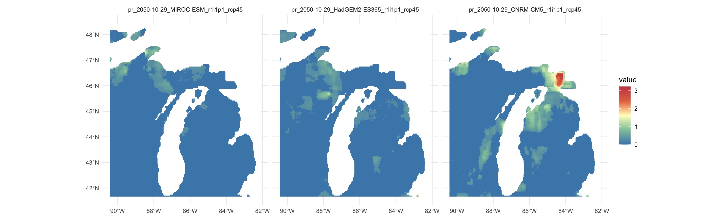
Getting multiple models results is also quite simple:

models = c("BNU-ESM","CanESM2", "CCSM4")

temp =  getMACA(AOI = aoi_get(state = "CO"),
                varname = 'tasmin', 
                model = models, 
                startDate = "2080-11-29")

temp =  c(temp[[1]], mean(temp[[1]]))

names(temp) = c(models, "Ensemble Mean")

If you don’t know your models, you can always grab a random set by specifying a number:

random = getMACA(aoi_get(state = "MI"), 
                 model = 3, 
                 varname = "pr", 
                 startDate = "2050-10-29")

Global Datasets

Not all datasets are USA focused either. TerraClimate offers global, monthly data up to the current year for many variables, and CHIRPS provides daily rainfall data:

kenya = aoi_get(country = "Kenya")
tc = getTerraClim(kenya, varname = "pet", startDate = "2018-01-01")
chirps = getCHIRPS(kenya, startDate = "2018-01-01", endDate = "2018-01-04" )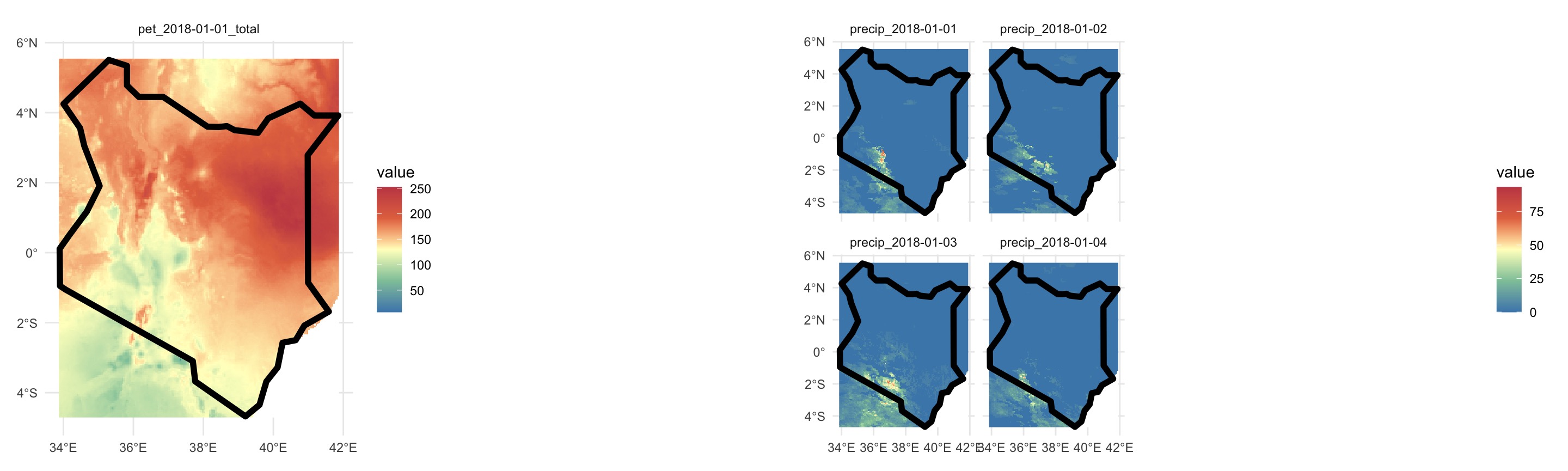

Point Based Data

Finally, data gathering is not limited to areal extents and can be retrieved as a time series at locations.

ts = data.frame(lng  = -105.0668, lat = 40.55085) %>% 
  st_as_sf(coords = c('lng', 'lat'), crs = 4326) %>% 
  getGridMET(varname =  c("pr", 'srad'), 
             startDate = "2021-01-01", 
             endDate = "2021-12-31")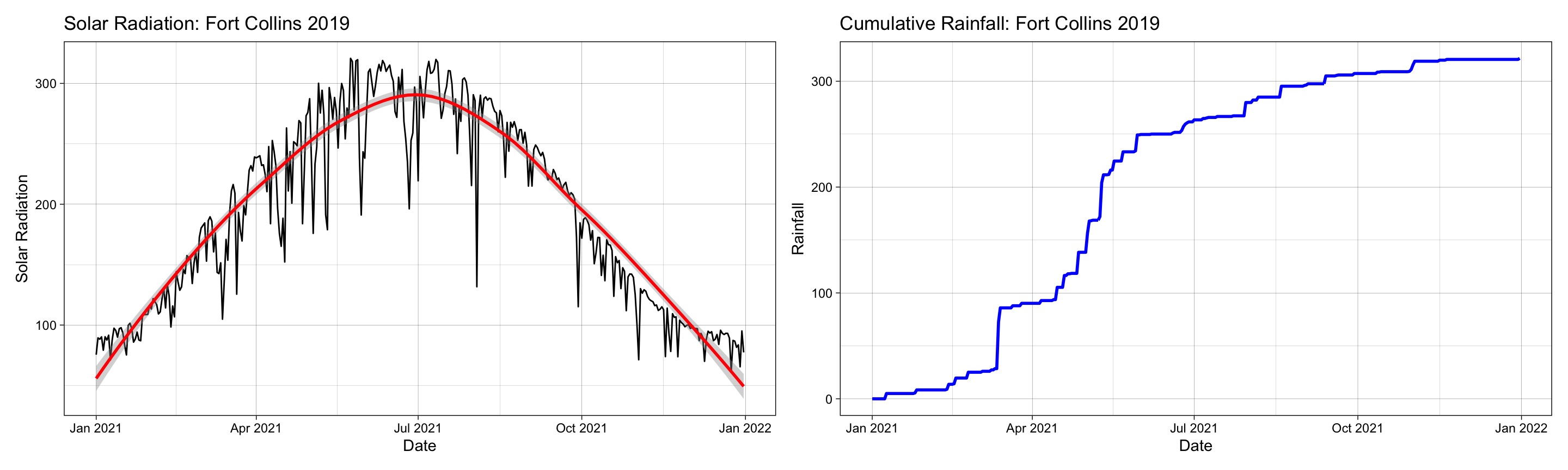

Point Based Ensemble

future = getMACA(geocode("Fort Collins", pt = TRUE), 
                 model = 5, 
                 varname = "tasmax", 
                 startDate = "2050-01-01", 
                 endDate = "2050-01-31")

future_long = pivot_longer(future, -date) 

ggplot(data = future_long, aes(x = date, y = value, col = name)) + 
  geom_line() + 
  theme_linedraw() + 
  scale_color_brewer(palette = "Dark2") + 
  labs(title = "Fort Collins Temperture: January, 2050",
       x = "Date",
       y = "Degree K",
       color = "Model")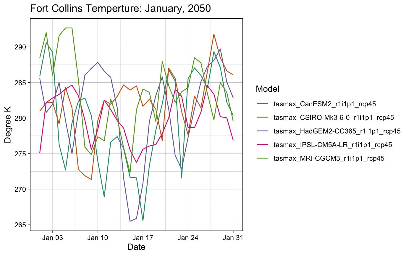

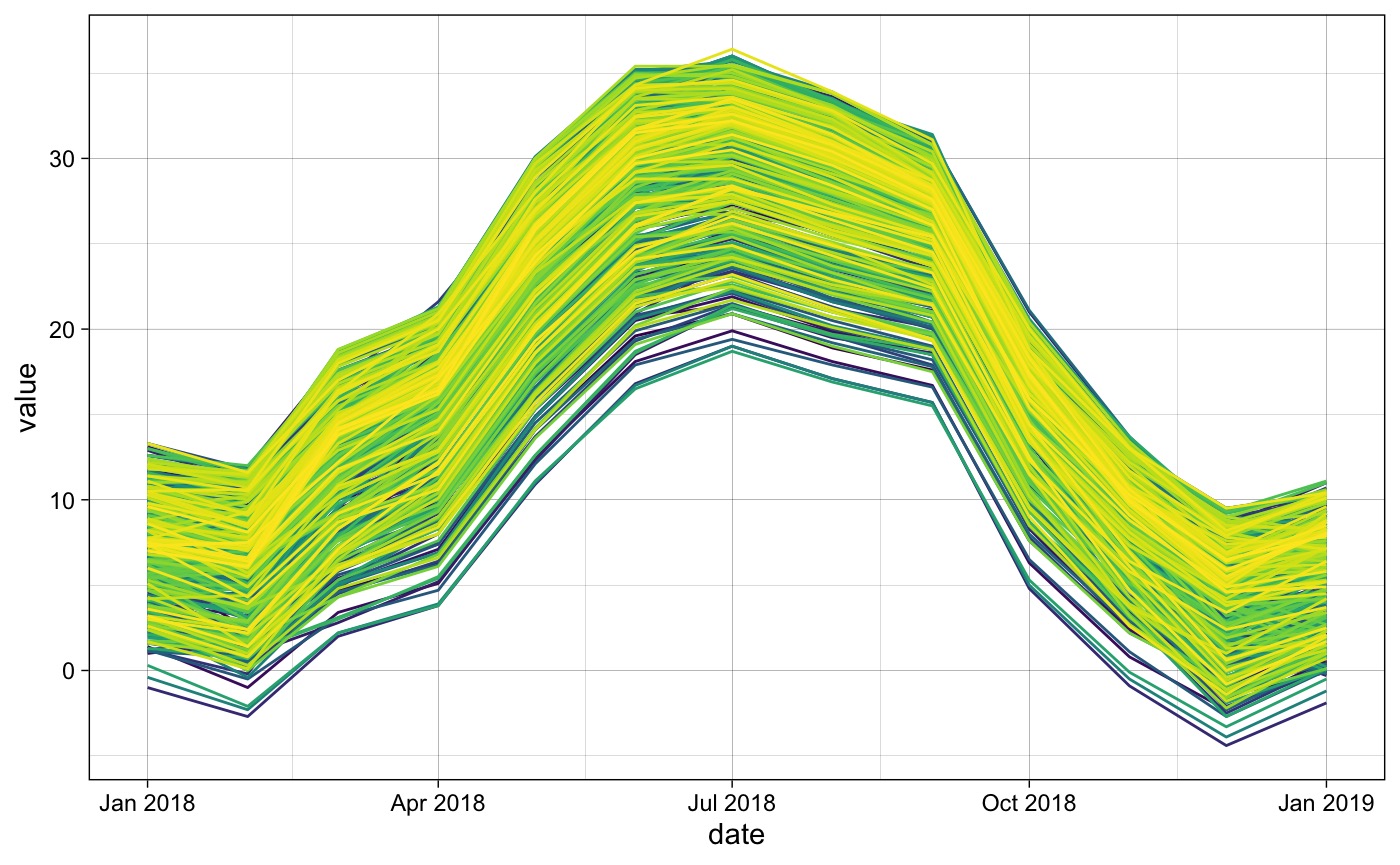
Multi site extraction

Extracting data for a set of points is an interesting challenge. It turns it is much more efficient to grab the underlying raster stack and then extract time series as opposed to iterating over the locations:

Starting with a set of locations in Colorado:

f = system.file("co/cities_colorado.rds", package = "climateR")
cities = readRDS(f)

climateR will grab the SpatRaster underlying the bounding area of the points

sites_stack = getTerraClim(AOI   = cities, 
                           varname = "tmax", 
                           startDate = "2018-01-01", 
                           endDate   = "2018-12-31")

Use extract_sites to extract the times series from these locations. The id parameter is the unique identifier from the site data with which to names the resulting columns.

sites_wide = extract_sites(r = sites_stack, pts = cities, ID = "NAME")
sites_wide[1:5, 1:5]
#>         date ADAMSCITY AGATE AGUILAR AKRON
#> 1 2018-01-01       9.5   8.2    11.4   7.1
#> 2 2018-02-01       8.1   7.1     9.9   5.8
#> 3 2018-03-01      14.6  14.1    15.0  13.5
#> 4 2018-04-01      17.5  16.6    17.6  16.2
#> 5 2018-05-01      25.1  25.0    25.5  24.8

To make the data ‘tidy’ simply pivot on the date column:

tmax = tidyr::pivot_longer(sites_wide, -date)
head(tmax)
#> # A tibble: 6 × 3
#>   date                name       value
#>   <dttm>              <chr>      <dbl>
#> 1 2018-01-01 00:00:00 ADAMSCITY   9.5 
#> 2 2018-01-01 00:00:00 AGATE       8.2 
#> 3 2018-01-01 00:00:00 AGUILAR    11.4 
#> 4 2018-01-01 00:00:00 AKRON       7.10
#> 5 2018-01-01 00:00:00 ALAMOSA     5.2 
#> 6 2018-01-01 00:00:00 ALLENSPARK  6.10

Mike Johnson