Lecture 16

Model Implementation & Workflow

Unit Example

Can we predict if a plot of land is forested? - Interested in classification models - We have a dataset of 7,107 6000-acre hexagons in Washington state. - Each hexagon has a nominal outcome, forested, with levels "Yes" and "No".

Data on forests in Washington

The U.S. Forest Service maintains ML models to predict whether a plot of land is “forested.”
This classification is important for all sorts of research, legislation, and land management purposes.
Plots are typically remeasured every 10 years and this dataset contains the most recent measurement per plot.
Type ?forested to learn more about this dataset, including references.

Data on forests in Washington

library(tidymodels)
library(forested)
dim(forested)
#> [1] 7107   19

One observation from each of 7,107 6000-acre hexagons in Washington state.
A nominal outcome, forested, with levels "Yes" and "No", measured “on-the-ground.”

table(forested$forested)
#> 
#>  Yes   No 
#> 3894 3213

18 remotely-sensed and easily-accessible predictors:

names(forested)
#>  [1] "forested"         "year"             "elevation"        "eastness"        
#>  [5] "northness"        "roughness"        "tree_no_tree"     "dew_temp"        
#>  [9] "precip_annual"    "temp_annual_mean" "temp_annual_min"  "temp_annual_max" 
#> [13] "temp_january_min" "vapor_min"        "vapor_max"        "canopy_cover"    
#> [17] "lon"              "lat"              "land_type"

Data splitting and spending

The initial split

set.seed(123)
forested_split <- initial_split(forested, prop = .8, strata = tree_no_tree)
forested_split
#> <Training/Testing/Total>
#> <5685/1422/7107>

Accessing the data

forested_train <- training(forested_split)
forested_test  <- testing(forested_split)

nrow(forested_train)
#> [1] 5685
nrow(forested_test)
#> [1] 1422

K-Fold Cross-Validation

# Load the dataset
set.seed(123)

# Create a 10-fold cross-validation object
(forested_folds <- vfold_cv(forested_train, v = 10))
#> #  10-fold cross-validation 
#> # A tibble: 10 × 2
#>    splits             id    
#>    <list>             <chr> 
#>  1 <split [5116/569]> Fold01
#>  2 <split [5116/569]> Fold02
#>  3 <split [5116/569]> Fold03
#>  4 <split [5116/569]> Fold04
#>  5 <split [5116/569]> Fold05
#>  6 <split [5117/568]> Fold06
#>  7 <split [5117/568]> Fold07
#>  8 <split [5117/568]> Fold08
#>  9 <split [5117/568]> Fold09
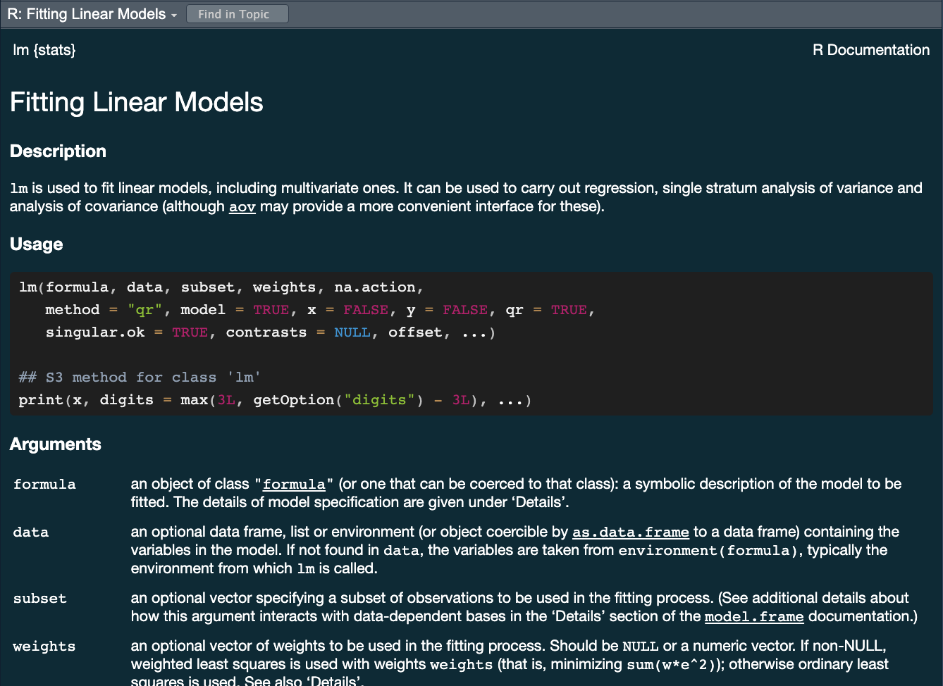
#> 10 <split [5117/568]> Fold10

How do you fit a linear model in R?

lm for linear model <– The one we have looked at!
glmnet for regularized regression
keras for regression using TensorFlow
stan for Bayesian regression using Stan
spark for large data sets using spark
brulee for regression using torch (PyTourch)

Challenge

All of these models have different syntax and functions
How do you keep track of all of them?
How do you know which one to use?
How would you compare them?

Comparing 3-5 of these models is a lot of work using functions for diverse packages.

The tidymodels advantage

In the tidymodels framework, all models are created using the same syntax:
- This makes it easy to compare models
- This makes it easy to switch between models
- This makes it easy to use the same model with different engines (packages)
The parsnip package provides a consistent interface to many models
For example, to fit a linear model you would be able to access the linear_reg() function

?linear_reg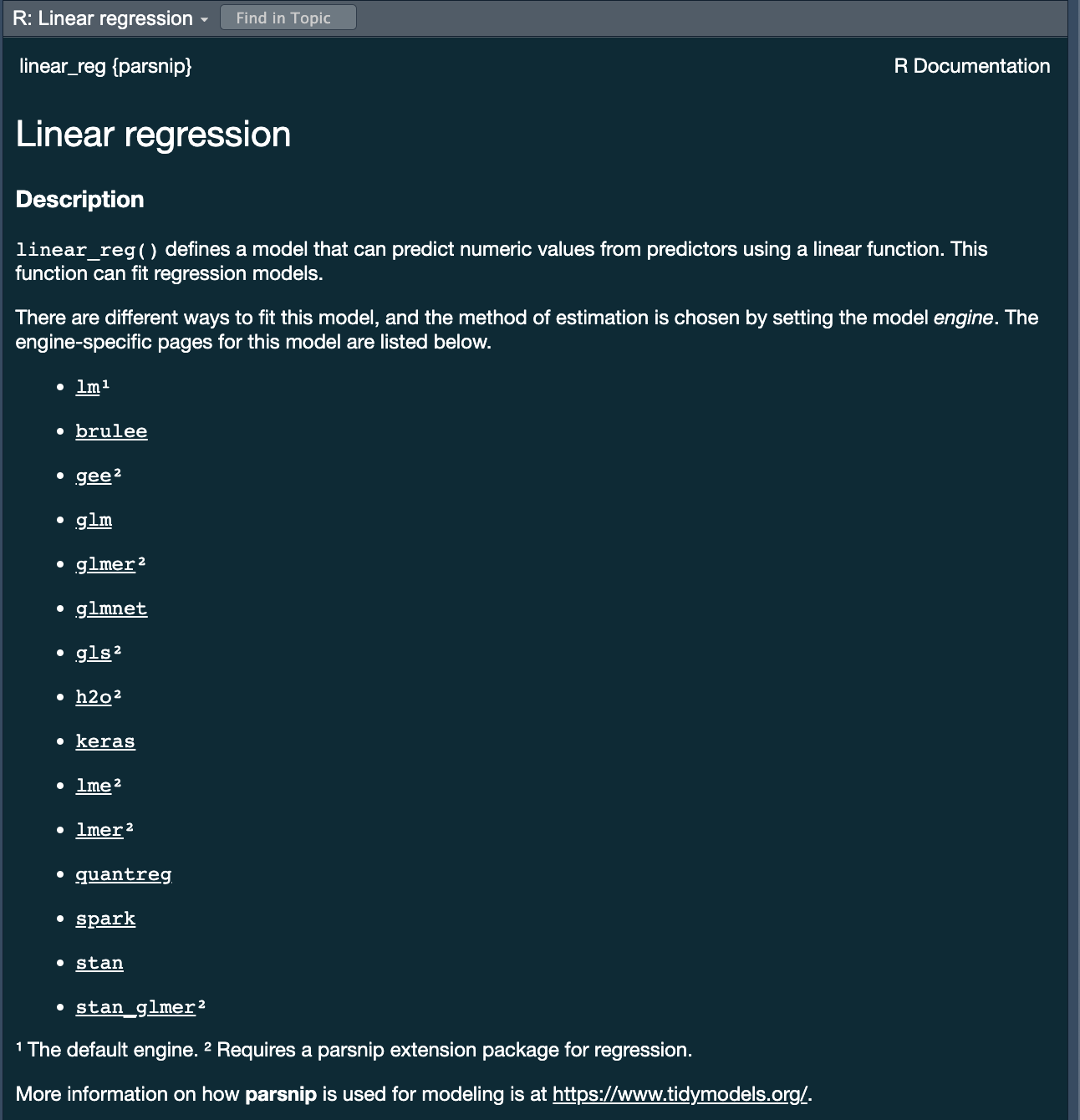

A tidymodels prediction will …

always be inside a tibble
have column names and types are unsurprising and predictable
ensure the number of rows in new_data and the output are the same

To specify a model

. . .

Choose a model
Specify an engine
Set the mode

Specify a model: Type

Next week we will discuss model types more thoroughly. For now, we will focus on two types:

Logistic Regression

logistic_reg()
#> Logistic Regression Model Specification (classification)
#> 
#> Computational engine: glm

decision_tree()
#> Decision Tree Model Specification (unknown mode)
#> 
#> Computational engine: rpart

We chose these two because they are robust, simple model that fit our goal of predicting a binary condition/class (forested/not forested)

Specify a model: engine

Choose a model
Specify an engine
Set the mode

?logistic_reg()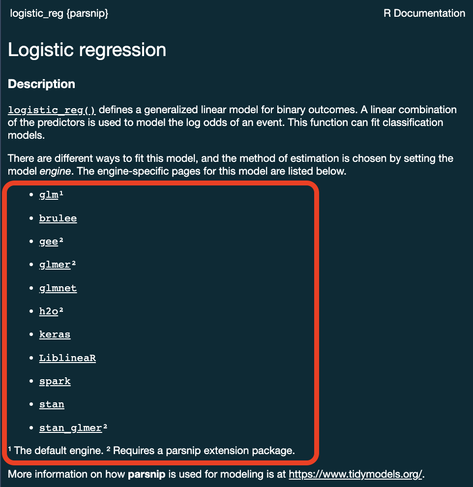

Specify a model: engine

logistic_reg() %>%
  set_engine("glmnet")
#> Logistic Regression Model Specification (classification)
#> 
#> Computational engine: glmnet

. . .

logistic_reg() %>%
  set_engine("stan")
#> Logistic Regression Model Specification (classification)
#> 
#> Computational engine: stan

Specify a model: mode

Choose a model
Specify an engine
Set the mode

?logistic_reg()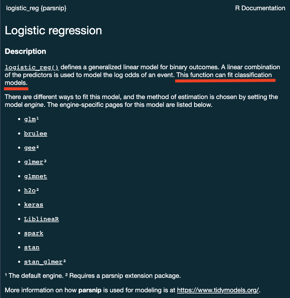

Specify a model: mode

Some models have limit classes …

logistic_reg() 
#> Logistic Regression Model Specification (classification)
#> 
#> Computational engine: glm

. . .

Others requires specification …

decision_tree()
#> Decision Tree Model Specification (unknown mode)
#> 
#> Computational engine: rpart

decision_tree() %>% 
  set_mode("classification")
#> Decision Tree Model Specification (classification)
#> 
#> Computational engine: rpart

All available models are listed at https://www.tidymodels.org/find/parsnip/

To specify a model

Choose a model
Specify an engine
Set the mode

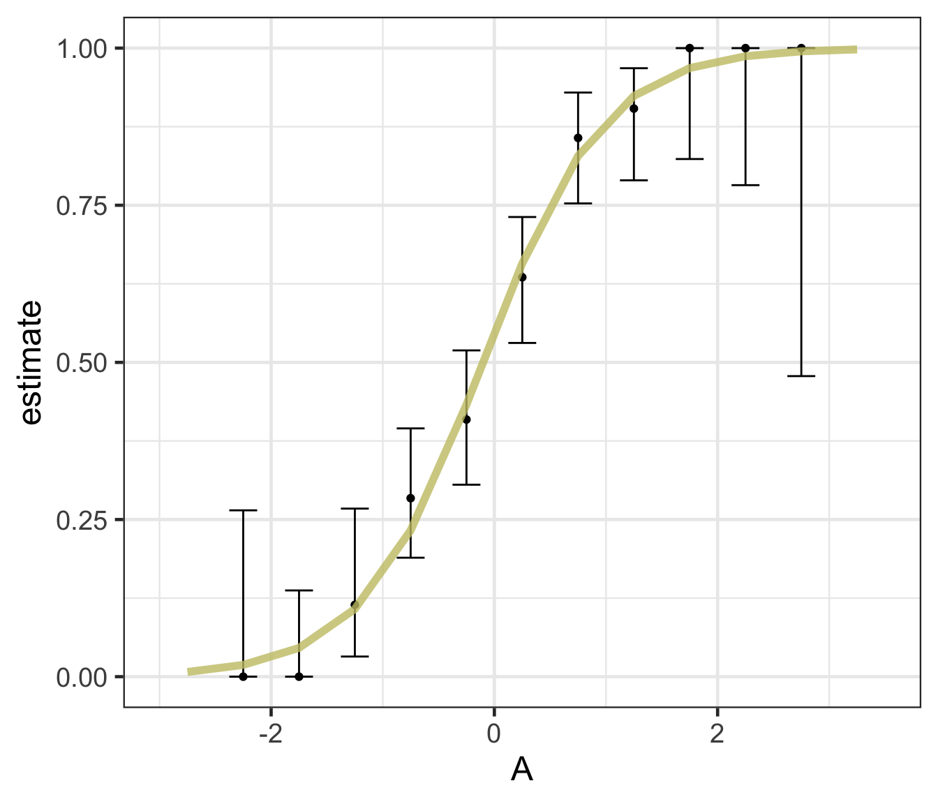
Logistic regression

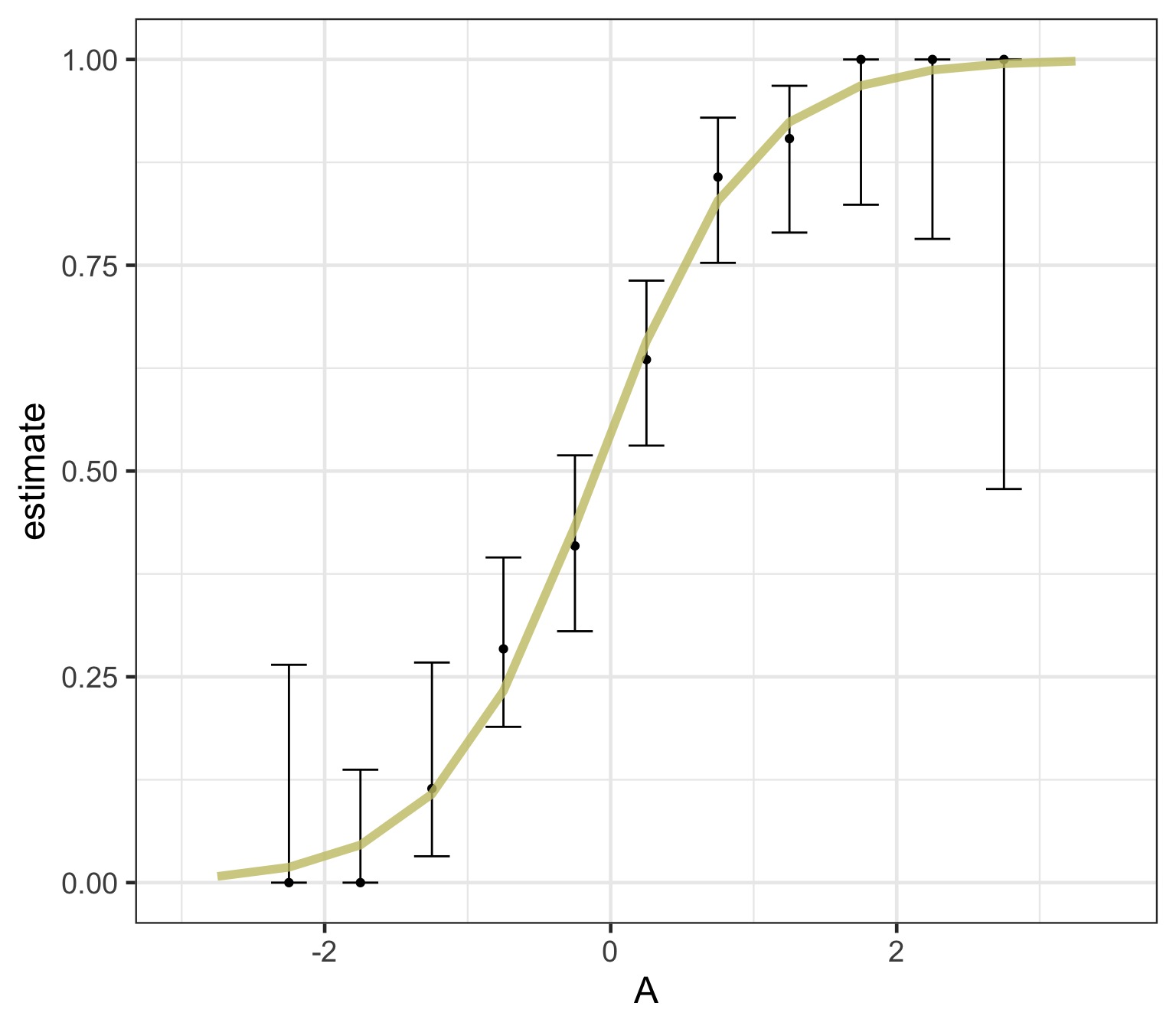
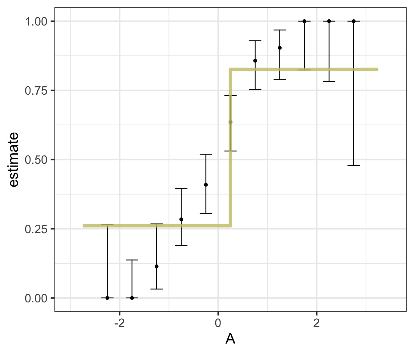
Logistic regression predicts probability—instead of a straight line, it gives an S-shaped curve that estimates how likely an outcome (e.g., is forested) is based on a predictor (e.g., rainfall and temperature).
The dots in the plot show the actual proportion of “successes” (e.g., is forested) within different bins of the predictor variable(s) (A).
The vertical error bars represent uncertainty—showing a range where the true probability might fall.
Logistic regression helps answer “how likely” questions—e.g., “How likely is someone to pass based on their study hours?” rather than just predicting a yes/no outcome.

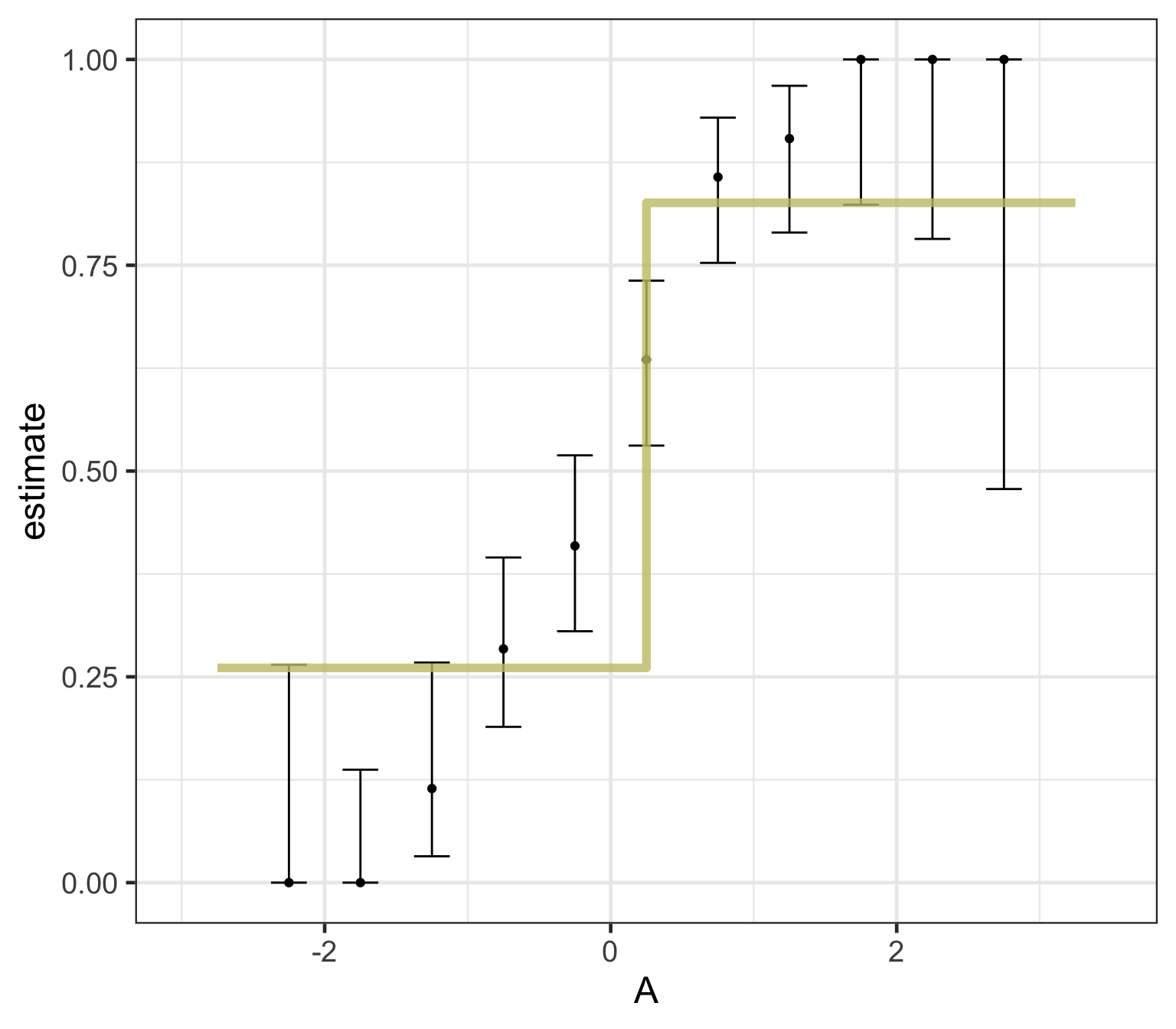
Decision trees

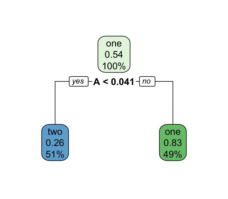
Decision trees

Series of splits or if/then statements based on predictors
First the tree grows until some condition is met (maximum depth, no more data)
Then the tree is pruned to reduce its complexity

Decision trees

What algorithm is best for estimate forested plots?

We can only really know by testing them …

Logistic regression

Decision trees

Fitting your model:

OK! So you have split data, you have a model, and you have an engine and mode
Now you need to fit the model!
This is done using the fit() function

dt_model <- decision_tree() %>% 
  set_engine('rpart') %>%
  set_mode("classification")

# Model, formula, data inputs
(output <- fit(dt_model, forested ~ ., data = forested_train) )
#> parsnip model object
#> 
#> n= 5685 
#> 
#> node), split, n, loss, yval, (yprob)
#>       * denotes terminal node
#> 
#>  1) root 5685 2571 Yes (0.54775726 0.45224274)  
#>    2) land_type=Tree 3025  289 Yes (0.90446281 0.09553719) *
#>    3) land_type=Barren,Non-tree vegetation 2660  378 No (0.14210526 0.85789474)  
#>      6) temp_annual_max< 13.395 351  155 Yes (0.55840456 0.44159544)  
#>       12) tree_no_tree=Tree 91    5 Yes (0.94505495 0.05494505) *
#>       13) tree_no_tree=No tree 260  110 No (0.42307692 0.57692308) *
#>      7) temp_annual_max>=13.395 2309  182 No (0.07882200 0.92117800) *

Component extracts:

While tidymodels provides a standard interface to all models all base models have specific methods (remember summary.lm? )
To use these, you must extract a the underlying object.
extract_fit_engine() extracts the underlying model object
extract_fit_parsnip() extracts the parsnip object
extract_recipe() extracts the recipe object
extract_preprocessor() extracts the preprocessor object
… many more

ex <- extract_fit_engine(output)
class(ex) # the class of the engine used!
#> [1] "rpart"

# Use rpart plot and text methods ...
plot(ex)
text(ex, cex = 0.9, use.n = TRUE, xpd = TRUE,)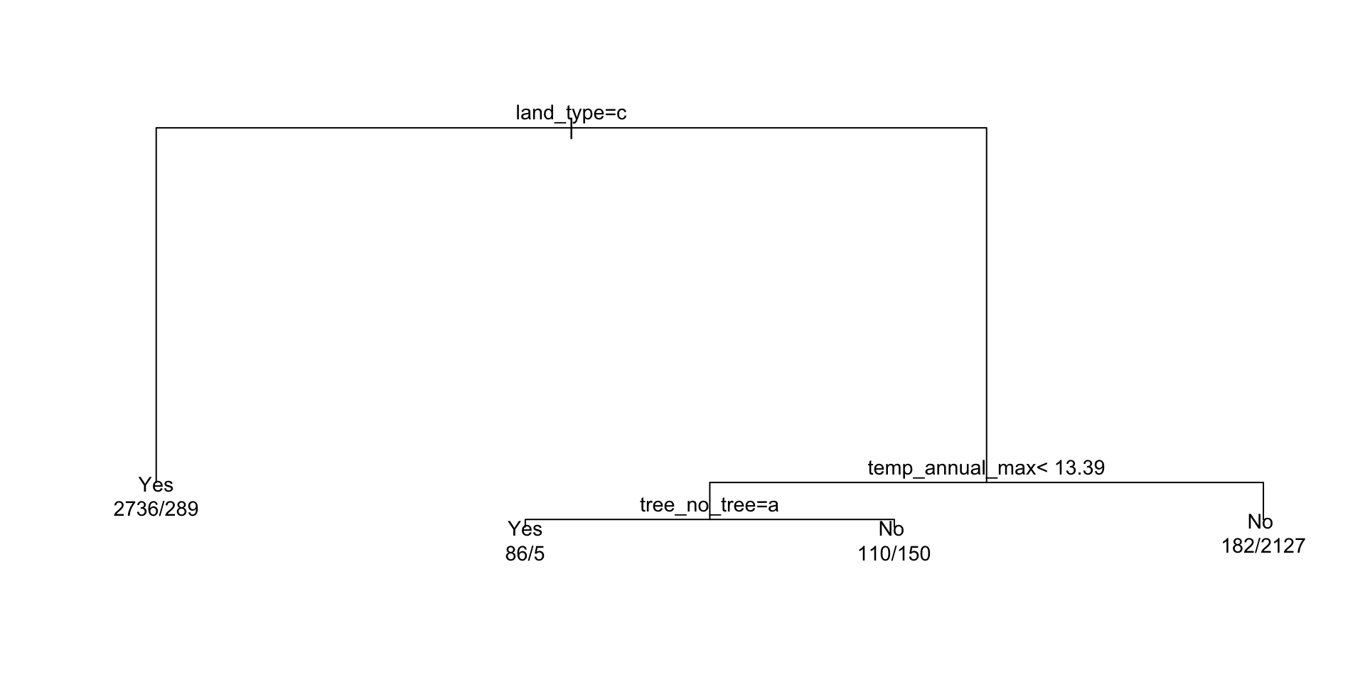

A model workflow

Workflows?

The workflows package in tidymodels helps:

Manage preprocessing and modeling in a structured pipeline
Avoid repetitive code
Reduce errors when integrating steps

. . .

Think of them as containers for:

Preprocessing steps (e.g., feature engineering, transformations)
Model specification
Fitting approaches

. . .

Why Use Workflows?

✅ Keeps preprocessing and modeling together

✅ Ensures consistency in data handling

✅ Makes code easier to read and maintain

Basic Workflow Structure:

Create a workflow object (similar to how ggplot() instantiates a canvas)
Add a formula or recipe (preprocessor)
Add the model
Fit the workflow

A model workflow

dt_wf <- workflow() %>%
  add_formula(forested ~ .) %>%
  add_model(dt_model) %>%
  fit(data = forested_train)

#> ══ Workflow [trained] ══════════════════════════════════════════════════════════
#> Preprocessor: Formula
#> Model: decision_tree()
#> 
#> ── Preprocessor ────────────────────────────────────────────────────────────────
#> forested ~ .
#> 
#> ── Model ───────────────────────────────────────────────────────────────────────
#> n= 5685 
#> 
#> node), split, n, loss, yval, (yprob)
#>       * denotes terminal node
#> 
#>  1) root 5685 2571 Yes (0.54775726 0.45224274)  
#>    2) land_type=Tree 3025  289 Yes (0.90446281 0.09553719) *
#>    3) land_type=Barren,Non-tree vegetation 2660  378 No (0.14210526 0.85789474)  
#>      6) temp_annual_max< 13.395 351  155 Yes (0.55840456 0.44159544)  
#>       12) tree_no_tree=Tree 91    5 Yes (0.94505495 0.05494505) *
#>       13) tree_no_tree=No tree 260  110 No (0.42307692 0.57692308) *
#>      7) temp_annual_max>=13.395 2309  182 No (0.07882200 0.92117800) *

Predict with your model

How do you use your new model?

augment() will return the dataset with predictions and residuals added.

dt_preds <- augment(dt_wf, new_data = forested_test)

#> # A tibble: 1,422 × 22
#>    .pred_class .pred_Yes .pred_No forested  year elevation eastness northness
#>    <fct>           <dbl>    <dbl> <fct>    <dbl>     <dbl>    <dbl>     <dbl>
#>  1 Yes            0.904    0.0955 No        2005       164      -84        53
#>  2 Yes            0.904    0.0955 Yes       2005       806       47       -88
#>  3 No             0.423    0.577  Yes       2005      2240      -67       -74
#>  4 Yes            0.904    0.0955 Yes       2005       787       66       -74
#>  5 Yes            0.904    0.0955 Yes       2005      1330       99         7
#>  6 Yes            0.904    0.0955 Yes       2005      1423       46        88
#>  7 Yes            0.904    0.0955 Yes       2014       546      -92       -38
#>  8 Yes            0.904    0.0955 Yes       2014      1612       30       -95
#>  9 No             0.0788   0.921  No        2014       235        0      -100
#> 10 No             0.0788   0.921  No        2014       308      -70       -70
#> # ℹ 1,412 more rows
#> # ℹ 14 more variables: roughness <dbl>, tree_no_tree <fct>, dew_temp <dbl>,
#> #   precip_annual <dbl>, temp_annual_mean <dbl>, temp_annual_min <dbl>,
#> #   temp_annual_max <dbl>, temp_january_min <dbl>, vapor_min <dbl>,
#> #   vapor_max <dbl>, canopy_cover <dbl>, lon <dbl>, lat <dbl>, land_type <fct>

Evaluate your model

How do you evaluate the skill of your models?

We will learn more about model evaluation and tuning latter in this unit, but for now we can blindly use the metrics() function defaults to get a sense of how our model is doing.

The default metrics for classification models are accuracy and kap (Cohen’s Kappa)
The default metric for regression models are RMSE, R^2, and MAE

# We have a classification model
metrics(dt_preds, truth = forested, estimate = .pred_class)
#> # A tibble: 2 × 3
#>   .metric  .estimator .estimate
#>   <chr>    <chr>          <dbl>
#> 1 accuracy binary         0.885
#> 2 kap      binary         0.768

`tidymodels` advantage!

OK! while that was not too much work, it certainly wasn’t minimal.

. . .

Now lets say you want to check if the logistic regression model performs better than the decision tree
That sounds like a lot to repeat.
Fortunately, the tidymodels framework makes this a straight forward swap!

. . .

log_mod = logistic_reg() %>% 
  set_engine("glm") %>% 
  set_mode("classification")

log_wf <- workflow() %>%
  add_formula(forested ~ .) %>%
  add_model(log_mod) %>%
  fit(data = forested_train)

log_preds <- augment(log_wf, new_data = forested_test)

metrics(log_preds, truth = forested, estimate = .pred_class)
#> # A tibble: 2 × 3
#>   .metric  .estimator .estimate
#>   <chr>    <chr>          <dbl>
#> 1 accuracy binary         0.890
#> 2 kap      binary         0.777

So who wins?

metrics(dt_preds, truth = forested, estimate = .pred_class)
#> # A tibble: 2 × 3
#>   .metric  .estimator .estimate
#>   <chr>    <chr>          <dbl>
#> 1 accuracy binary         0.885
#> 2 kap      binary         0.768
metrics(log_preds, truth = forested, estimate = .pred_class)
#> # A tibble: 2 × 3
#>   .metric  .estimator .estimate
#>   <chr>    <chr>          <dbl>
#> 1 accuracy binary         0.890
#> 2 kap      binary         0.777

Right out of the gate, there doesn’t seem to be much difference, but …

Don’t get to confident!

We have evaluated the model on the same data we trained it on
This is not a good practice and can give us a false sense of confidence
Instead, we can use our resamples to better understand the skill of a model based on the iterative leave out policy:

dt_wf_rs <- workflow() %>%
  add_formula(forested ~ .) %>%
  add_model(dt_model) %>%
  fit_resamples(resamples = forested_folds, 
                # Here we just ask tidymodels to save all predictions...
                control   = control_resamples(save_pred = TRUE))

#> # A tibble: 1 × 5
#>   splits             id     .metrics         .notes           .predictions      
#>   <list>             <chr>  <list>           <list>           <list>            
#> 1 <split [5116/569]> Fold01 <tibble [3 × 4]> <tibble [0 × 3]> <tibble [569 × 6]>

Note

tidyr::unnest could be used to expand any of those list columns!

Don’t get to confident!

We can execute the same workflow for the logistic regression model, this time evaluating the resamples instead of the test data.

log_wf_rs <- workflow() %>%
  add_formula(forested ~ .) %>%
  add_model(log_mod) %>%
  fit_resamples(resamples = forested_folds,
                control = control_resamples(save_pred = TRUE))

#> # Resampling results
#> # 10-fold cross-validation 
#> # A tibble: 10 × 5
#>    splits             id     .metrics         .notes           .predictions
#>    <list>             <chr>  <list>           <list>           <list>      
#>  1 <split [5116/569]> Fold01 <tibble [3 × 4]> <tibble [0 × 3]> <tibble>    
#>  2 <split [5116/569]> Fold02 <tibble [3 × 4]> <tibble [0 × 3]> <tibble>    
#>  3 <split [5116/569]> Fold03 <tibble [3 × 4]> <tibble [0 × 3]> <tibble>    
#>  4 <split [5116/569]> Fold04 <tibble [3 × 4]> <tibble [0 × 3]> <tibble>    
#>  5 <split [5116/569]> Fold05 <tibble [3 × 4]> <tibble [0 × 3]> <tibble>    
#>  6 <split [5117/568]> Fold06 <tibble [3 × 4]> <tibble [0 × 3]> <tibble>    
#>  7 <split [5117/568]> Fold07 <tibble [3 × 4]> <tibble [0 × 3]> <tibble>    
#>  8 <split [5117/568]> Fold08 <tibble [3 × 4]> <tibble [0 × 3]> <tibble>    
#>  9 <split [5117/568]> Fold09 <tibble [3 × 4]> <tibble [0 × 3]> <tibble>    
#> 10 <split [5117/568]> Fold10 <tibble [3 × 4]> <tibble [0 × 3]> <tibble>

Don’t get to confident!

Since we now have an “ensemble” of models (across the folds), we can collect a summary of the metrics across them.
The default metrics for classification ensembles are:
- accuracy: accuracy is the proportion of correct predictions
- brier_class: the Brier score for classification is the mean squared difference between the predicted probability and the actual outcome
- roc_auc: the area under the ROC (Receiver Operating Characteristic) curve


collect_metrics(log_wf_rs)
#> # A tibble: 3 × 6
#>   .metric     .estimator   mean     n std_err .config             
#>   <chr>       <chr>       <dbl> <int>   <dbl> <chr>               
#> 1 accuracy    binary     0.906     10 0.00360 Preprocessor1_Model1
#> 2 brier_class binary     0.0714    10 0.00191 Preprocessor1_Model1
#> 3 roc_auc     binary     0.961     10 0.00164 Preprocessor1_Model1
collect_metrics(dt_wf_rs)
#> # A tibble: 3 × 6
#>   .metric     .estimator   mean     n std_err .config             
#>   <chr>       <chr>       <dbl> <int>   <dbl> <chr>               
#> 1 accuracy    binary     0.896     10 0.00385 Preprocessor1_Model1
#> 2 brier_class binary     0.0889    10 0.00224 Preprocessor1_Model1
#> 3 roc_auc     binary     0.909     10 0.00267 Preprocessor1_Model1

Further simplification: `workflowsets`

OK, so we have streamlined a lot of things with tidymodels:

We have a specified preprocesser (e.g. formula or recipe)
We have defined a model (complete with engine and mode)
We have implemented workflows pairing each model with the preprocesser to either fit the model to the resamples, or, the training data.

While a significant improvement, we can do better!

Does the idea of implementing a process over an list of elements ring a bell?

Model mappings:

workflowsets is a package that builds off of purrr and allows you to iterate over multiple models and/or multiple resamples
Remember how map, map_*, map2, and walk2 functions allow lists to map to lists or vectors? workflow_set maps a preprocessor (formula or recipe) to a set of models - each provided as a list object.
To start, we will create a workflow_set object (instead of a workflow). The first argument is a list of preprocessor objects (formulas or recipes) and the second argument is a list of model objects.
Both must be lists, by nature of the underlying purrr code.

(wf_obj <- workflow_set(list(forested ~.), list(log_mod, dt_model)))
#> # A workflow set/tibble: 2 × 4
#>   wflow_id              info             option    result    
#>   <chr>                 <list>           <list>    <list>    
#> 1 formula_logistic_reg  <tibble [1 × 4]> <opts[0]> <list [0]>
#> 2 formula_decision_tree <tibble [1 × 4]> <opts[0]> <list [0]>

Iteritive extecution

Once the workflow_set object is created, the workflow_map function can be used to map a function across the preprocessor/model combinations.
Here we are mapping the fit_resamples function across the workflow_set combinations using the resamples argument to specify the resamples we want to use (forested_folds).

wf_obj <- 
  workflow_set(list(forested ~.), list(log_mod, dt_model)) %>%
  workflow_map("fit_resamples", resamples = forested_folds)

#> # A workflow set/tibble: 2 × 4
#>   wflow_id              info             option    result   
#>   <chr>                 <list>           <list>    <list>   
#> 1 formula_logistic_reg  <tibble [1 × 4]> <opts[1]> <rsmp[+]>
#> 2 formula_decision_tree <tibble [1 × 4]> <opts[1]> <rsmp[+]>

Rapid comparision

With that single function, all models have been fit to the resamples and we can quickly compare the results both graphically and statistically:

# Quick plot function
autoplot(wf_obj) + 
  theme_linedraw()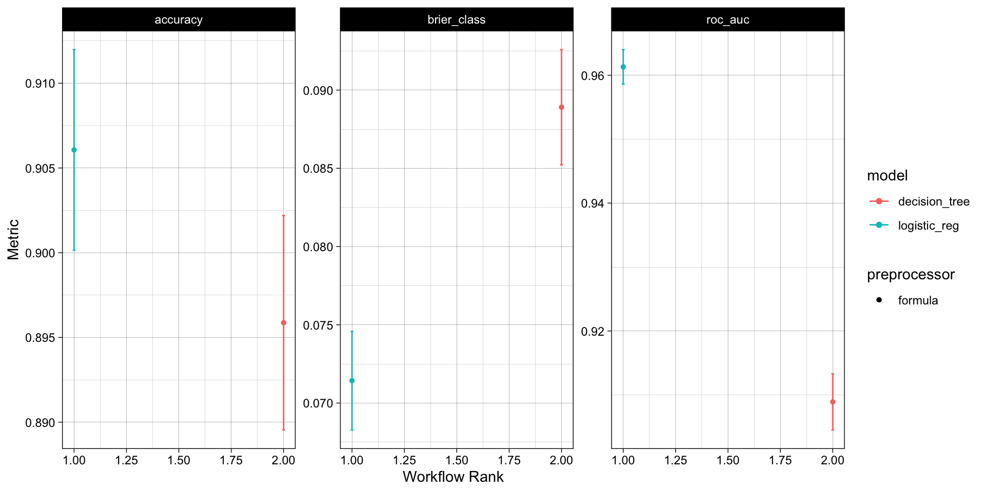

# Long list of results, ranked by accuracy
rank_results(wf_obj, 
            rank_metric = "accuracy", 
            select_best = TRUE)
#> # A tibble: 6 × 9
#>   wflow_id         .config .metric   mean std_err     n preprocessor model  rank
#>   <chr>            <chr>   <chr>    <dbl>   <dbl> <int> <chr>        <chr> <int>
#> 1 formula_logisti… Prepro… accura… 0.906  0.00360    10 formula      logi…     1
#> 2 formula_logisti… Prepro… brier_… 0.0714 0.00191    10 formula      logi…     1
#> 3 formula_logisti… Prepro… roc_auc 0.961  0.00164    10 formula      logi…     1
#> 4 formula_decisio… Prepro… accura… 0.896  0.00385    10 formula      deci…     2
#> 5 formula_decisio… Prepro… brier_… 0.0889 0.00224    10 formula      deci…     2
#> 6 formula_decisio… Prepro… roc_auc 0.909  0.00267    10 formula      deci…     2

. . .

Overall, the logistic regression model appears to the best model for this data set!

The whole game - status update

Next Monday, we’ll talk more about models we can chose from.
Next Wednesday, we’ll have an in-class demo of this whole process.

Assignment

Open your R script from the last daily assignment
Add a new section for the model fitting and workflow
Define a logistic regression model and a rand_forest model

rand_forest is new, so, think about the engine (use the default) and mode needed for our problem

Set up a workflow_set() to compare the logistic regression model (the winner of lecture here) to the rand_forest model you create. Use accuracy as you primary metric to rank the models.
As a comment, write a sentence about what model you think is best!
Submit your R script to Canvas

Unit Example

Data on forests in Washington

Data on forests in Washington

Data splitting and spending

The initial split

Accessing the data

K-Fold Cross-Validation

How do you fit a linear model in R?

Challenge

The tidymodels advantage

A tidymodels prediction will …

To specify a model

Specify a model: Type

Specify a model: engine

Specify a model: engine

Specify a model: mode

Specify a model: mode

Some models have limit classes …

Others requires specification …

To specify a model

Logistic regression

Decision trees

Decision trees

Decision trees

What algorithm is best for estimate forested plots?

Logistic regression

Decision trees

Fitting your model:

Component extracts:

A model workflow

Workflows?

Basic Workflow Structure:

A model workflow

Predict with your model

Evaluate your model

tidymodels advantage!

So who wins?

Don’t get to confident!

Don’t get to confident!

Don’t get to confident!

Further simplification: workflowsets

Model mappings:

Iteritive extecution

Rapid comparision

The whole game - status update

Assignment

`tidymodels` advantage!

Further simplification: `workflowsets`