Lecture 02
The Digital Environment
2025-02-09
Slido!

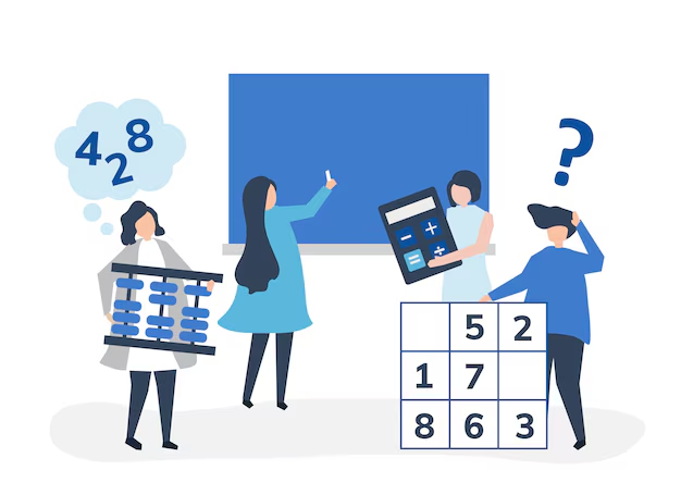
Quantitative Reasoning
Working Definition:
Thinking about *data* from our world, to better understand and make choices about the past, present and future.Many people can work with data (e.g., data scientists), many people have domain knowledge (e.g., hydrologists), but few can do both in a careful way. That’s the goal of this class!
Almost all data is digital.
Working with computers is essential for quantitative analysis (precursor to reasoning).
Today is all about understanding how we interface with computers, their strengths, and limitations.
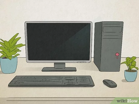
Your Environment
Computer: An electronic device for storing and processing data, typically in binary form, according to instruction. Computers store persistent data on disk, ephemeral data in memory, and executes processes with the CPU (Central Processing Unit).
File: A block of arbitrary information available to a computer program.

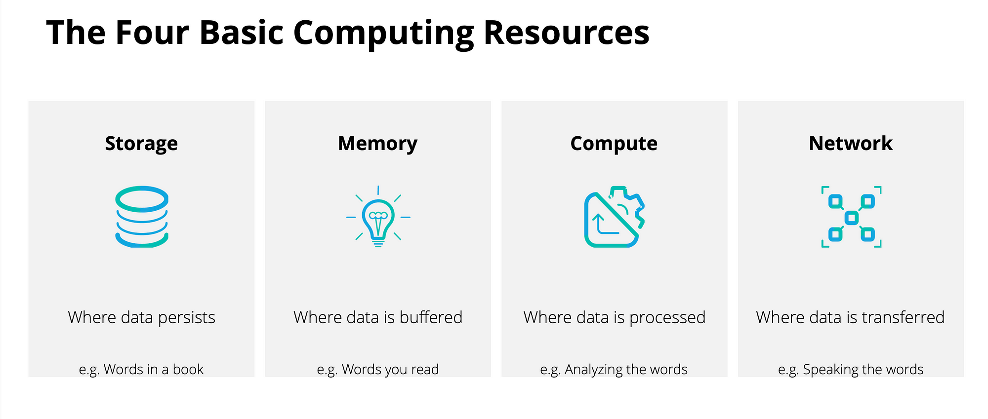
Compute
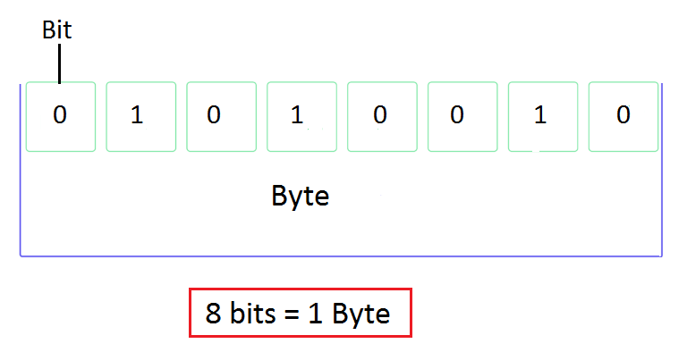
Bytes vs Bits
A byte is a group of 8 binary digits (bits) and a unit of memory size.
The bit is a basic unit of information in computing and represents a logical state with two possible values (0 or 1).
File Storage
- Files are stored as a collection of bytes on a hard drive
- Hard drives do not understand files - they just store bytes and directions to those bytes
- We need ways to retrieve (and write) bytes from (and to) the hard drive.
Interpreting Capacity

New computer capacity
Storage Pattern
File Storage
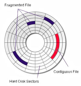
Defragmentation

What is a file?
Files save data on the hard drive as bytes in a meaningful way.
Files have three key properties:
- a name (machine and human interpret-able address)
- a path (a location in the file system)
- an extension (how to/what program reads the format)

Filesystem
Tip
For every file, there are paths and directories that lead to that specific file. These paths and directories are called File Systems.
Filesystem: describes the methods an operating system uses to organize files
If you are on a Windows device , and you want to find a file you just downloaded, you go to “This PC,” from where you click on “Documents” and there you find yet another folder called “Downloads” that has the downloaded files stored.
If you are on a Mac , to get the same result is click on “Downloads.” Whether you do it from the menu bar or anywhere else, it’s going to get you to exactly where you need to go.
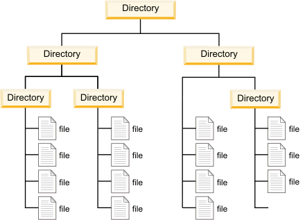
Directories
Directory: is a location for storing, organizing, and separating files and other directories on a computer. Think of folders!
Root directory: the “highest” or top-level directory in the hierarchy.
- The root directory contains all other folders/files in the drive or folder
- Sometimes referred to as the home directory
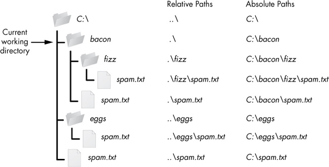
File Paths
File paths tell us the location of a file within the file system
Directories are stored as hierarchies, again with root (home) directory being the one holding everything on a system
The folder you are in, is called your working directory. (think
pwd)The folder above the working directory is the parent directory
All folders within the working directory are sub folders or child folder
.. and . notation
The dot (.) and dot-dot (..) notation to help us write shorter paths
A single ‘.’ denotes “this directory”.
Two periods (“..”) means “the parent directory”
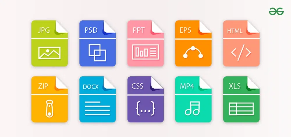
File Extensions
All files store bits.
Extensions can be considered a type of metadata that provides information about the way data might be stored
There are 1000’s of different formats for data ranging from common to custom
Each format defines how the sequence of bits and bytes are laid out
Indicate the characteristics of the file, its intended use, and the default applications that can open/use the file.
If you double click a
.docxfile it opens in Word which interprets the meaning of the bytesIf you double click an
.Rfile it opens with RStudio, and R interprets the meaning of the bytes
Extension Interpretation
- Readers depended on anticipated structure
- The file is actually a PNG with the wrong file extension. “0x89 0x50” is how a PNG file starts.
- The data returned to R is a structured set of bits, interpreted according to the directions of the file and the interpreting language!

Structure
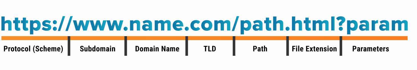
- Protocol (Scheme): https, ftp, s3, …
- Subdomain
- Domain Name
- Top Level Domain (TLD)
- Path/File (w/ extension!)
- Parameters (APIs, databases, etc.)
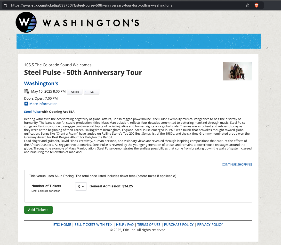
Information
https://www.etix.com/ticket/p/53375671/steel-pulse-50th-anniversary-tour-fort-collins-washingtons
Important
index.html is everywhere online (lets take a look!)
Summary:
Next Time:
Daily Assignment: Set up Git and Github
Next Topic: Data Types