Week 1

Expectations / Level Setting

🚀 Getting Started with R for Data Science

Welcome to 523C: Environmental Data Science Applications: Water Resources!
This first lecture will introduce essential, high-level topics to help you build a strong foundation in R for environmental data science.
Throughout the lecture, you will be asked to assess your comfort level with various topics via a Google survey.
The survey results will help tailor the course focus, ensuring that we reinforce challenging concepts while avoiding unnecessary review of familiar topics.

Google Survey

Please open this survey and answer the questions as we work through this lecture.
Your responses will provide valuable insights into areas where additional explanations or hands-on exercises may be beneficial.

Google Survey

~ Week 1: Data Science Basics

Data Types

R has five principal data types (excluding raw and complex):

Character: A string of text, represented with quotes (e.g., “hello”).
- Used to store words, phrases, and categorical data.
Integer: A whole number, explicitly defined with an L suffix (e.g., 42L).
- Stored more efficiently than numeric values when decimals are not needed.
Numeric: A floating-point number, used for decimal values (e.g., 3.1415).
- This is the default type for numbers in R.
Boolean (Logical): A logical value that represents TRUE or FALSE.
- Commonly used in logical operations and conditional statements.

character <- "a"
integer <- 1L
numeric <- 3.3
boolean <- TRUE

Data Structures

When working with multiple values, we need data structures to store and manipulate data efficiently.
R provides several types of data structures, each suited for different use cases.

Vector

A vector is the most basic data structure in R and contains elements of the same type.
Vectors are created using the c() function.

char.vec <- c("a", "b", "c")
boolean.vec <- c(TRUE, FALSE, TRUE)

Lists allow for heterogeneous data types.

list <- list(a = c(1,2,3),
            b = c(TRUE, FALSE),
            c = "test")

Matrix

# Creating a sequence of numbers:
(vec <- 1:9)
#> [1] 1 2 3 4 5 6 7 8 9

A matrix is a two-dimensional data structure where a diminision (dim) is added to an atomic vector
Matrices are created using the matrix() function.

# Default column-wise filling
matrix(vec, nrow = 3)
#>      [,1] [,2] [,3]
#> [1,]    1    4    7
#> [2,]    2    5    8
#> [3,]    3    6    9

# Row-wise filling
matrix(vec, nrow = 3, byrow = TRUE)
#>      [,1] [,2] [,3]
#> [1,]    1    2    3
#> [2,]    4    5    6
#> [3,]    7    8    9

Array

An array extends matrices to higher dimensions.
It is useful when working with multi-dimensional data.

# Creating a 2x2x2 array
array(vec, dim = c(2,2,2))
#> , , 1
#> 
#>      [,1] [,2]
#> [1,]    1    3
#> [2,]    2    4
#> 
#> , , 2
#> 
#>      [,1] [,2]
#> [1,]    5    7
#> [2,]    6    8

Data Frame / Tibble

Data Frames: A table-like (rectangular) structure where each column is a vector of equal length.
- Used for storing datasets where different columns can have different data types.
Tibble: A modern version of a data frame that supports list-columns and better printing.
- Offers improved performance and formatting for large datasets.

(df  <- data.frame(char.vec, boolean.vec))
#>   char.vec boolean.vec
#> 1        a        TRUE
#> 2        b       FALSE
#> 3        c        TRUE

(tib <- tibble::tibble(char.vec, list))
#> # A tibble: 3 × 2
#>   char.vec list        
#>   <chr>    <named list>
#> 1 a        <dbl [3]>   
#> 2 b        <lgl [2]>   
#> 3 c        <chr [1]>

📦 Installing Packages

R has a vast ecosystem of packages that extend its capabilities both on CRAN and github
To install a package from CRAN, use install.packages().
To install a package from Github, use remotes::install_github()`.
We’ll start by installing palmerpenguins, which contains a dataset on penguins.

install.packages('palmerpenguins')

Attaching/Loading Packages

To use an installed package, you need to load it in your current working session using library().
Here, we load palmerpenguins for dataset exploration and tidyverse for data science workflows.

library(palmerpenguins) # 🐧 Fun dataset about penguins!
library(tidyverse)      # 🛠 Essential for data science in R

Help & Documentation

R has built-in documentation that provides information about functions and datasets.
To access documentation, use ?function_name.
Example: Viewing the help page for the penguins dataset.

?penguins

You can also use help.search("keyword") to look up topics of interest.
For vignettes (detailed guides), use vignette("package_name").

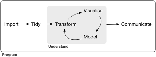
Quarto: Communication

In this class we will use Quarto, a more modern, cross langauge version of Rmarkdown
If you are comfortable with Rmd, you’ll quickly be able to transition to Qmd
If you are new to Rmd, you’ll be able to learn the latest and greatest

🌟 Tidyverse: A Swiss Army Knife for Data Science R

The tidyverse is a collection of packages designed for data science.
We can see what it includes using the tidyverse_packages function:

tidyverse_packages()
#>  [1] "broom"         "conflicted"    "cli"           "dbplyr"       
#>  [5] "dplyr"         "dtplyr"        "forcats"       "ggplot2"      
#>  [9] "googledrive"   "googlesheets4" "haven"         "hms"          
#> [13] "httr"          "jsonlite"      "lubridate"     "magrittr"     
#> [17] "modelr"        "pillar"        "purrr"         "ragg"         
#> [21] "readr"         "readxl"        "reprex"        "rlang"        
#> [25] "rstudioapi"    "rvest"         "stringr"       "tibble"       
#> [29] "tidyr"         "xml2"          "tidyverse"

While all tidyverse packages are valuable, the main ones we will focus on are:

readr: Reading data
tibble: Enhanced data frames
dplyr: Data manipulation
tidyr: Data reshaping
purrr: Functional programming
ggplot2: Visualization

Combined, this provides us a complete “data science” toolset:

readr

The readr package provides functions for reading data into R.
The read_csv() function reads comma-separated files.
The read_tsv() function reads tab-separated files.
The read_delim() function reads files with custom delimiters.
In all cases, more intellegent parsing is done than with base R equivalents.

read_csv

path = 'https://raw.githubusercontent.com/mikejohnson51/csu-ess-330/refs/heads/main/resources/county-centroids.csv'

# base R
read.csv(path) |> 
  head()
#>    fips        LON      LAT
#> 1  1061  -85.83575 31.09404
#> 2  8125 -102.42587 40.00307
#> 3 17177  -89.66239 42.35138
#> 4 28153  -88.69577 31.64132
#> 5 34041  -74.99570 40.85940
#> 6 46051  -96.76981 45.17255

# More inutitive readr
read_csv(path) |> 
  head()
#> # A tibble: 6 × 3
#>   fips     LON   LAT
#>   <chr>  <dbl> <dbl>
#> 1 01061  -85.8  31.1
#> 2 08125 -102.   40.0
#> 3 17177  -89.7  42.4
#> 4 28153  -88.7  31.6
#> 5 34041  -75.0  40.9
#> 6 46051  -96.8  45.2

dplyr

The dplyr package provides functions for data manipulation throuhg ‘a grammar for data manipulation’.
It provides capabilities similar to SQL for data manipulation.
It includes functions for viewing, filtering, selecting, mutating, summarizing, and joining data.

`%>%` / `|>`

The pipe operator %>% is used to chain operations in R.
The pipe operator |> is a base R version of %>% introduced in R 4.1.
The pipe passes what on the “left hand” side to the function on the “right hand” side as the first argument.

penguins |> 
  glimpse()
#> Rows: 344
#> Columns: 8
#> $ species           <fct> Adelie, Adelie, Adelie, Adelie, Adelie, Adelie, Adel…
#> $ island            <fct> Torgersen, Torgersen, Torgersen, Torgersen, Torgerse…
#> $ bill_length_mm    <dbl> 39.1, 39.5, 40.3, NA, 36.7, 39.3, 38.9, 39.2, 34.1, …
#> $ bill_depth_mm     <dbl> 18.7, 17.4, 18.0, NA, 19.3, 20.6, 17.8, 19.6, 18.1, …
#> $ flipper_length_mm <int> 181, 186, 195, NA, 193, 190, 181, 195, 193, 190, 186…
#> $ body_mass_g       <int> 3750, 3800, 3250, NA, 3450, 3650, 3625, 4675, 3475, …
#> $ sex               <fct> male, female, female, NA, female, male, female, male…
#> $ year              <int> 2007, 2007, 2007, 2007, 2007, 2007, 2007, 2007, 2007…

glimpse

The glimpse() function provides a concise summary of a dataset.

glimpse(penguins)
#> Rows: 344
#> Columns: 8
#> $ species           <fct> Adelie, Adelie, Adelie, Adelie, Adelie, Adelie, Adel…
#> $ island            <fct> Torgersen, Torgersen, Torgersen, Torgersen, Torgerse…
#> $ bill_length_mm    <dbl> 39.1, 39.5, 40.3, NA, 36.7, 39.3, 38.9, 39.2, 34.1, …
#> $ bill_depth_mm     <dbl> 18.7, 17.4, 18.0, NA, 19.3, 20.6, 17.8, 19.6, 18.1, …
#> $ flipper_length_mm <int> 181, 186, 195, NA, 193, 190, 181, 195, 193, 190, 186…
#> $ body_mass_g       <int> 3750, 3800, 3250, NA, 3450, 3650, 3625, 4675, 3475, …
#> $ sex               <fct> male, female, female, NA, female, male, female, male…
#> $ year              <int> 2007, 2007, 2007, 2007, 2007, 2007, 2007, 2007, 2007…

select

The select() function is used to select columns from a dataset.
It is useful when you want to work with specific columns.
Example: Selecting the species column from the penguins dataset.

select(penguins, species)
#> # A tibble: 344 × 1
#>    species
#>    <fct>  
#>  1 Adelie 
#>  2 Adelie 
#>  3 Adelie 
#>  4 Adelie 
#>  5 Adelie 
#>  6 Adelie 
#>  7 Adelie 
#>  8 Adelie 
#>  9 Adelie 
#> 10 Adelie 
#> # ℹ 334 more rows

filter

The filter() function is used to filter rows based on a condition.
It is useful when you want to work with specific rows.
Example: Filtering the penguins dataset to include only Adelie penguins.

filter(penguins, species == "Adelie")
#> # A tibble: 152 × 8
#>    species island    bill_length_mm bill_depth_mm flipper_length_mm body_mass_g
#>    <fct>   <fct>              <dbl>         <dbl>             <int>       <int>
#>  1 Adelie  Torgersen           39.1          18.7               181        3750
#>  2 Adelie  Torgersen           39.5          17.4               186        3800
#>  3 Adelie  Torgersen           40.3          18                 195        3250
#>  4 Adelie  Torgersen           NA            NA                  NA          NA
#>  5 Adelie  Torgersen           36.7          19.3               193        3450
#>  6 Adelie  Torgersen           39.3          20.6               190        3650
#>  7 Adelie  Torgersen           38.9          17.8               181        3625
#>  8 Adelie  Torgersen           39.2          19.6               195        4675
#>  9 Adelie  Torgersen           34.1          18.1               193        3475
#> 10 Adelie  Torgersen           42            20.2               190        4250
#> # ℹ 142 more rows
#> # ℹ 2 more variables: sex <fct>, year <int>

mutate

The mutate() function is used to create new columns or modify existing ones.
It is useful when you want to add new information to your dataset.
Example: Creating a new column bill_length_cm from bill_length_mm.

Note the use of the tidy_select helper starts_with

mutate(penguins, bill_length_cm = bill_length_mm / 100) |> 
  select(starts_with("bill"))
#> # A tibble: 344 × 3
#>    bill_length_mm bill_depth_mm bill_length_cm
#>             <dbl>         <dbl>          <dbl>
#>  1           39.1          18.7          0.391
#>  2           39.5          17.4          0.395
#>  3           40.3          18            0.403
#>  4           NA            NA           NA    
#>  5           36.7          19.3          0.367
#>  6           39.3          20.6          0.393
#>  7           38.9          17.8          0.389
#>  8           39.2          19.6          0.392
#>  9           34.1          18.1          0.341
#> 10           42            20.2          0.42 
#> # ℹ 334 more rows

summarize

The summarize() function is used to aggregate data.
It is useful when you want to calculate summary statistics.
It always produces a one-row output.
Example: Calculating the mean bill_length_mm for all penguins

summarize(penguins, bill_length_mm = mean(bill_length_mm, na.rm = TRUE))
#> # A tibble: 1 × 1
#>   bill_length_mm
#>            <dbl>
#> 1           43.9

group_by / ungroup

The group_by() function is used to group data by one or more columns.
It is useful when you want to perform operations on groups.
It does this by adding a grouped_df class to the dataset.
The ungroup() function removes grouping from a dataset.

groups <- group_by(penguins, species)

dplyr::group_keys(groups)
#> # A tibble: 3 × 1
#>   species  
#>   <fct>    
#> 1 Adelie   
#> 2 Chinstrap
#> 3 Gentoo
dplyr::group_indices(groups)[1:5]
#> [1] 1 1 1 1 1

Group operations

Example: Grouping the penguins dataset by species and calculating the mean bill_length_mm.

penguins |> 
  group_by(species) |> 
  summarize(bill_length_mm = mean(bill_length_mm, na.rm = TRUE)) |> 
  ungroup()
#> # A tibble: 3 × 2
#>   species   bill_length_mm
#>   <fct>              <dbl>
#> 1 Adelie              38.8
#> 2 Chinstrap           48.8
#> 3 Gentoo              47.5

Joins

The dplyr package provides functions for joining datasets.
Common join functions include inner_join(), left_join(), right_join(), and full_join().
Joins are used to combine datasets based on shared keys (primary and foreign).

Mutating joins

Mutating joins add columns from one dataset to another based on a shared key.
Example: Adding species information to the penguins dataset based on the species_id.

species <- tribble(
  ~species_id, ~species,
  1, "Adelie",
  2, "Chinstrap",
  3, "Gentoo"
)

left_join

select(penguins, species, contains('bill')) |> 
  left_join(species, by = "species")
#> # A tibble: 344 × 4
#>    species bill_length_mm bill_depth_mm species_id
#>    <chr>            <dbl>         <dbl>      <dbl>
#>  1 Adelie            39.1          18.7          1
#>  2 Adelie            39.5          17.4          1
#>  3 Adelie            40.3          18            1
#>  4 Adelie            NA            NA            1
#>  5 Adelie            36.7          19.3          1
#>  6 Adelie            39.3          20.6          1
#>  7 Adelie            38.9          17.8          1
#>  8 Adelie            39.2          19.6          1
#>  9 Adelie            34.1          18.1          1
#> 10 Adelie            42            20.2          1
#> # ℹ 334 more rows

right_join

select(penguins, species, contains('bill')) |> 
  right_join(species, by = "species")
#> # A tibble: 344 × 4
#>    species bill_length_mm bill_depth_mm species_id
#>    <chr>            <dbl>         <dbl>      <dbl>
#>  1 Adelie            39.1          18.7          1
#>  2 Adelie            39.5          17.4          1
#>  3 Adelie            40.3          18            1
#>  4 Adelie            NA            NA            1
#>  5 Adelie            36.7          19.3          1
#>  6 Adelie            39.3          20.6          1
#>  7 Adelie            38.9          17.8          1
#>  8 Adelie            39.2          19.6          1
#>  9 Adelie            34.1          18.1          1
#> 10 Adelie            42            20.2          1
#> # ℹ 334 more rows

inner_join

select(penguins, species, contains('bill')) |> 
  right_join(species, by = "species")
#> # A tibble: 344 × 4
#>    species bill_length_mm bill_depth_mm species_id
#>    <chr>            <dbl>         <dbl>      <dbl>
#>  1 Adelie            39.1          18.7          1
#>  2 Adelie            39.5          17.4          1
#>  3 Adelie            40.3          18            1
#>  4 Adelie            NA            NA            1
#>  5 Adelie            36.7          19.3          1
#>  6 Adelie            39.3          20.6          1
#>  7 Adelie            38.9          17.8          1
#>  8 Adelie            39.2          19.6          1
#>  9 Adelie            34.1          18.1          1
#> 10 Adelie            42            20.2          1
#> # ℹ 334 more rows

full_join

select(penguins, species, contains('bill')) |> 
  right_join(species, by = "species")
#> # A tibble: 344 × 4
#>    species bill_length_mm bill_depth_mm species_id
#>    <chr>            <dbl>         <dbl>      <dbl>
#>  1 Adelie            39.1          18.7          1
#>  2 Adelie            39.5          17.4          1
#>  3 Adelie            40.3          18            1
#>  4 Adelie            NA            NA            1
#>  5 Adelie            36.7          19.3          1
#>  6 Adelie            39.3          20.6          1
#>  7 Adelie            38.9          17.8          1
#>  8 Adelie            39.2          19.6          1
#>  9 Adelie            34.1          18.1          1
#> 10 Adelie            42            20.2          1
#> # ℹ 334 more rows

Filtering Joins

Filtering joins retain only rows that match between datasets.
Example: Filtering the penguins dataset to include only rows with matching species_id.

select(penguins, species, contains('bill')) |> 
  semi_join(species, by = "species")
#> # A tibble: 344 × 3
#>    species bill_length_mm bill_depth_mm
#>    <fct>            <dbl>         <dbl>
#>  1 Adelie            39.1          18.7
#>  2 Adelie            39.5          17.4
#>  3 Adelie            40.3          18  
#>  4 Adelie            NA            NA  
#>  5 Adelie            36.7          19.3
#>  6 Adelie            39.3          20.6
#>  7 Adelie            38.9          17.8
#>  8 Adelie            39.2          19.6
#>  9 Adelie            34.1          18.1
#> 10 Adelie            42            20.2
#> # ℹ 334 more rows

ggplot2: Visualization

The ggplot2 package is used for data visualization.
It is based on the “grammar of graphics”, which allows for a high level of customization.
ggplot2 is built on the concept of layers, where each layer adds a different element to the plot.

`ggplot`

The ggplot() function initializes a plot.
It provides a blank canvas to which layers can be added.

ggplot()

data / aesthetics

Data must be provided to ggplot()
The aes() function is used to map variables to aesthetics (e.g., x and y axes).
aes arguments provided in ggplot are inherited by all layers.
Example: Creating a plot of body_mass_g vs. bill_length_mm.

ggplot(penguins, aes(x = body_mass_g, y = bill_length_mm))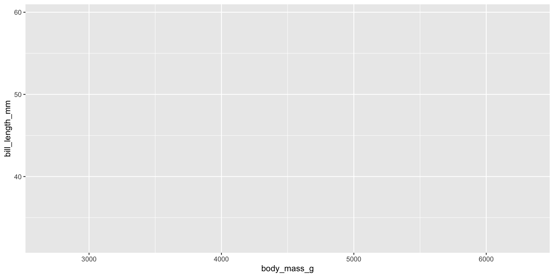

geom_*

The geom_*() functions add geometric objects to the plot.
They describe how to render the mapping created in aes
Example: Adding points to the plot.

ggplot(penguins, aes(x = body_mass_g, y = bill_length_mm)) + 
  geom_point()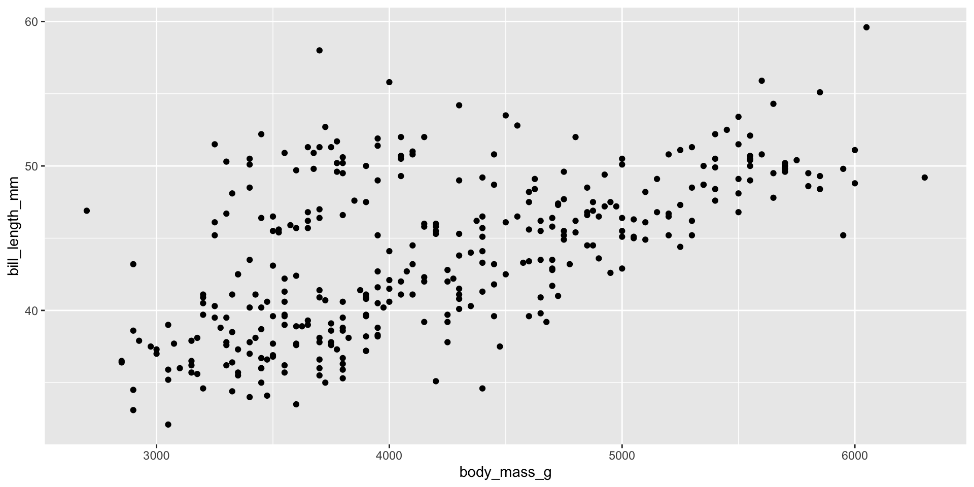

facet_wrap / facet_grid

The facet_wrap() function is used to create small multiples of a plot.
It is useful when you want to compare subsets of data.
The facet_grid() function is used to create a grid of plots.
Example: Faceting the plot by species.

ggplot(penguins, aes(x = body_mass_g, y = bill_length_mm)) + 
  geom_point() + 
  facet_wrap(~species)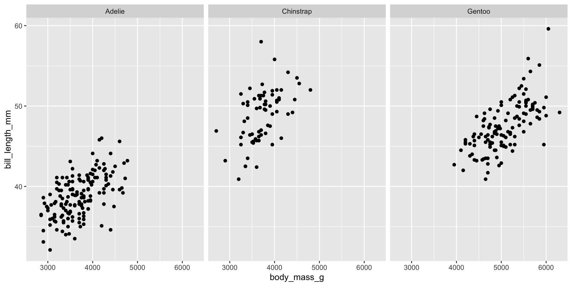

theme_*

The theme_*() functions are used to customize the appearance of the plot.
They allow you to modify the plot’s background, gridlines, and text.
Example: Applying the theme_linedraw() theme to the plot.

ggplot(penguins, aes(x = body_mass_g, y = bill_length_mm)) + 
  geom_point() + 
  facet_wrap(~species) + 
  theme_linedraw()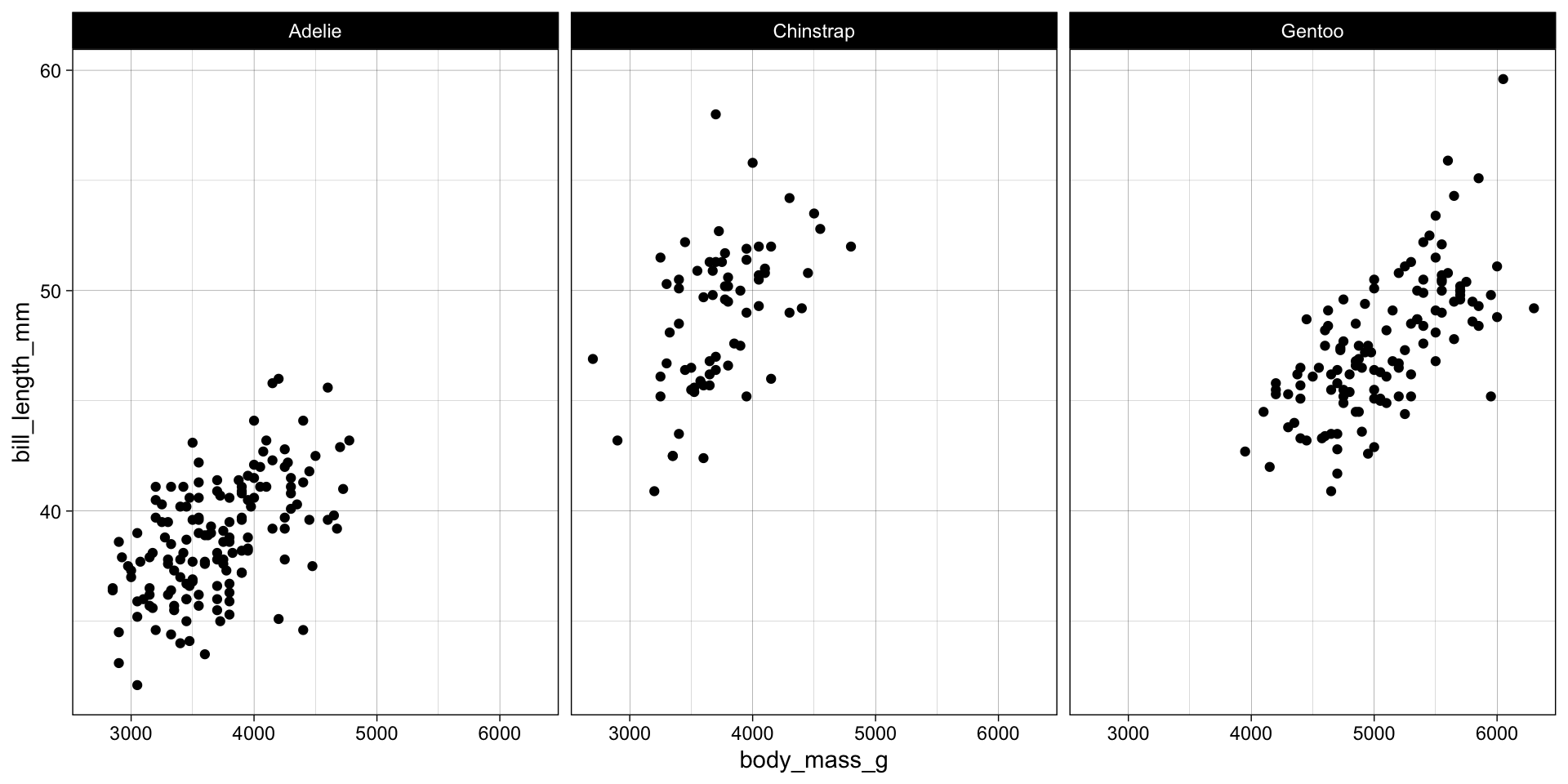

There are 1000s of themes available in the ggplot2 ecosystem
- ggthemes
- ggpubr
- hrbrthemes
- ggsci
- …

ggplot(penguins, aes(x = body_mass_g, y = bill_length_mm)) + 
  geom_point() + 
  facet_wrap(~species) + 
  ggthemes::theme_economist()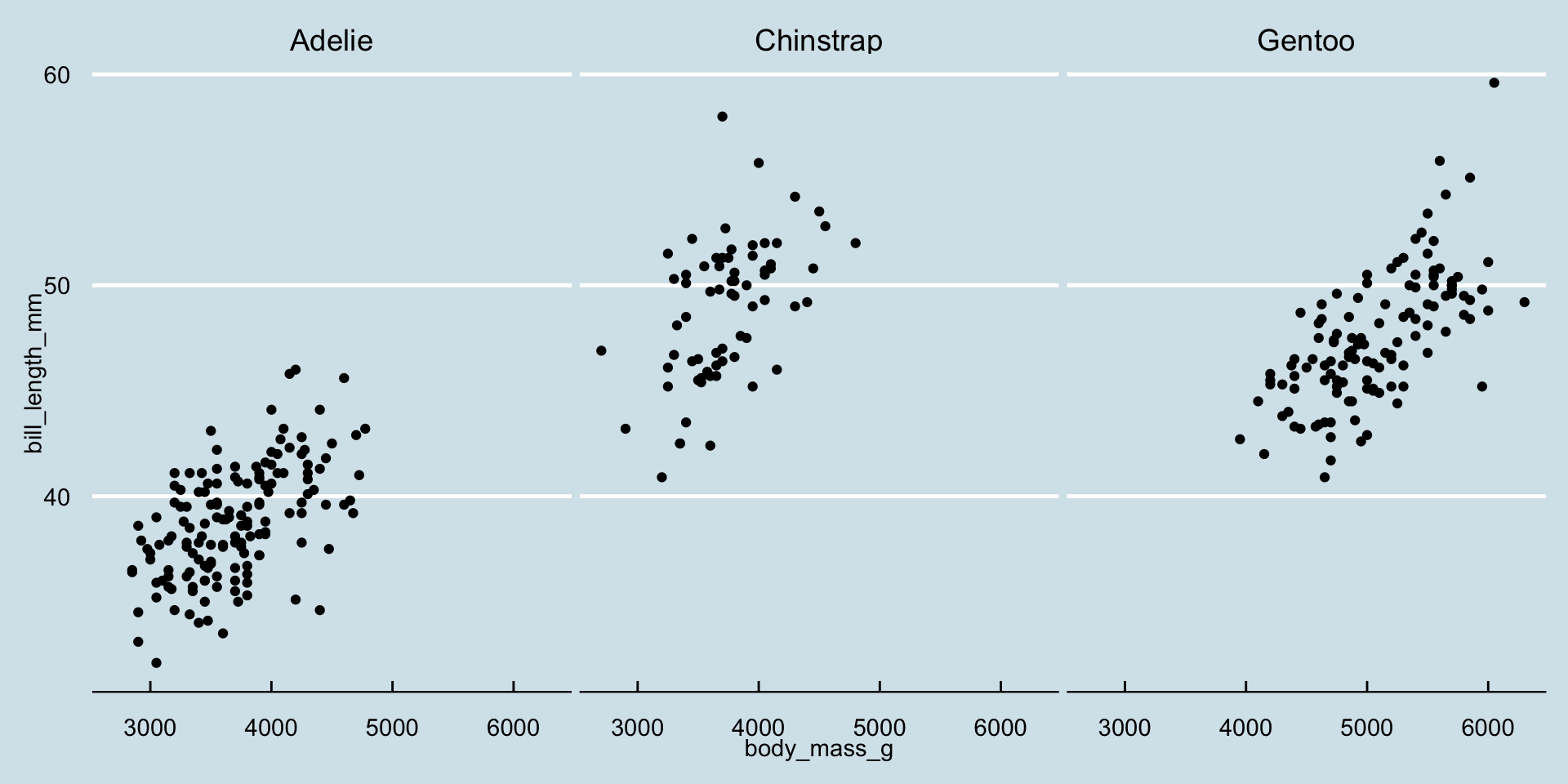

labs

The labs() function is used to add titles, subtitles, and axis labels to the plot.
It is useful for providing context and making the plot more informative.
Example: Adding titles and axis labels to the plot.

ggplot(penguins, aes(x = body_mass_g, y = bill_length_mm)) + 
  geom_point() + 
  facet_wrap(~species) + 
  theme_linedraw() + 
  labs(title = "Penguins Weight by Bill Size", 
       x = "Body Mass",
       y = "Bill Length", 
       subtitle = "Made for 523c")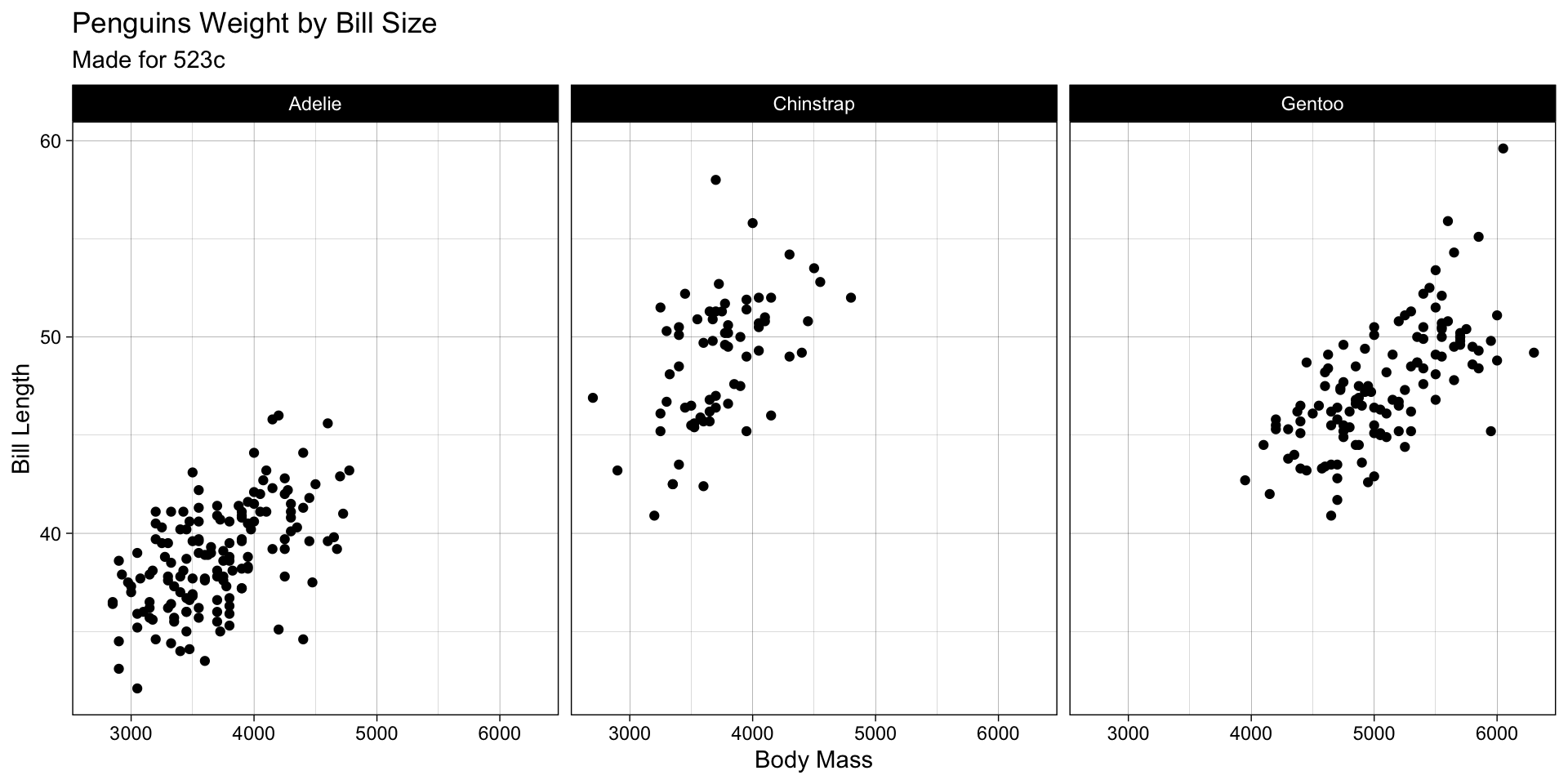

`tidyr`

The tidyr package provides functions for data reshaping.
It includes functions for pivoting and nesting data.

pivot_longer

The pivot_longer() function is used to convert wide data to long data.
It is useful when you want to work with data in a tidy format.
Example: Converting the penguins dataset from wide to long format.

(data.long = penguins |> 
  select(species, bill_length_mm, body_mass_g) |> 
  mutate(penguin_id = 1:n()) |> 
  pivot_longer(-c(penguin_id, species), 
               names_to = "Measure", 
               values_to = "value"))
#> # A tibble: 688 × 4
#>    species penguin_id Measure         value
#>    <fct>        <int> <chr>           <dbl>
#>  1 Adelie           1 bill_length_mm   39.1
#>  2 Adelie           1 body_mass_g    3750  
#>  3 Adelie           2 bill_length_mm   39.5
#>  4 Adelie           2 body_mass_g    3800  
#>  5 Adelie           3 bill_length_mm   40.3
#>  6 Adelie           3 body_mass_g    3250  
#>  7 Adelie           4 bill_length_mm   NA  
#>  8 Adelie           4 body_mass_g      NA  
#>  9 Adelie           5 bill_length_mm   36.7
#> 10 Adelie           5 body_mass_g    3450  
#> # ℹ 678 more rows

pivot_wider

The pivot_wider() function is used to convert long data to wide data.
It is useful when you want to work with data in a wide format.
Example: Converting the data.long dataset from long to wide format.

data.long |> 
  pivot_wider(names_from = "Measure", 
              values_from = "value")
#> # A tibble: 344 × 4
#>    species penguin_id bill_length_mm body_mass_g
#>    <fct>        <int>          <dbl>       <dbl>
#>  1 Adelie           1           39.1        3750
#>  2 Adelie           2           39.5        3800
#>  3 Adelie           3           40.3        3250
#>  4 Adelie           4           NA            NA
#>  5 Adelie           5           36.7        3450
#>  6 Adelie           6           39.3        3650
#>  7 Adelie           7           38.9        3625
#>  8 Adelie           8           39.2        4675
#>  9 Adelie           9           34.1        3475
#> 10 Adelie          10           42          4250
#> # ℹ 334 more rows

nest / unnest

The nest() function is used to nest data into a list-column.
It is useful when you want to group data together.
Example: Nesting the penguins dataset by species.

penguins |> 
  nest(data = -species)
#> # A tibble: 3 × 2
#>   species   data              
#>   <fct>     <list>            
#> 1 Adelie    <tibble [152 × 7]>
#> 2 Gentoo    <tibble [124 × 7]>
#> 3 Chinstrap <tibble [68 × 7]>

penguins |> 
  nest(data = -species) |> 
  unnest(data)
#> # A tibble: 344 × 8
#>    species island    bill_length_mm bill_depth_mm flipper_length_mm body_mass_g
#>    <fct>   <fct>              <dbl>         <dbl>             <int>       <int>
#>  1 Adelie  Torgersen           39.1          18.7               181        3750
#>  2 Adelie  Torgersen           39.5          17.4               186        3800
#>  3 Adelie  Torgersen           40.3          18                 195        3250
#>  4 Adelie  Torgersen           NA            NA                  NA          NA
#>  5 Adelie  Torgersen           36.7          19.3               193        3450
#>  6 Adelie  Torgersen           39.3          20.6               190        3650
#>  7 Adelie  Torgersen           38.9          17.8               181        3625
#>  8 Adelie  Torgersen           39.2          19.6               195        4675
#>  9 Adelie  Torgersen           34.1          18.1               193        3475
#> 10 Adelie  Torgersen           42            20.2               190        4250
#> # ℹ 334 more rows
#> # ℹ 2 more variables: sex <fct>, year <int>

linear modeling: lm

The lm() function is used to fit linear models.
It is useful when you want to model the relationship between two variables.
Example: Fitting a linear model to predict body_mass_g from flipper_length_mm.

model <- lm(body_mass_g ~ flipper_length_mm, data = drop_na(penguins))

summary(model)
#> 
#> Call:
#> lm(formula = body_mass_g ~ flipper_length_mm, data = drop_na(penguins))
#> 
#> Residuals:
#>      Min       1Q   Median       3Q      Max 
#> -1057.33  -259.79   -12.24   242.97  1293.89 
#> 
#> Coefficients:
#>                   Estimate Std. Error t value Pr(>|t|)    
#> (Intercept)       -5872.09     310.29  -18.93   <2e-16 ***
#> flipper_length_mm    50.15       1.54   32.56   <2e-16 ***
#> ---
#> Signif. codes:  0 '***' 0.001 '**' 0.01 '*' 0.05 '.' 0.1 ' ' 1
#> 
#> Residual standard error: 393.3 on 331 degrees of freedom
#> Multiple R-squared:  0.7621, Adjusted R-squared:  0.7614 
#> F-statistic:  1060 on 1 and 331 DF,  p-value: < 2.2e-16

broom

The broom package is used to tidy model outputs.
It provides functions to convert model outputs into tidy data frames.
Example: Tidying the model output.

tidy

The tidy() function is used to tidy model coefficients.
It is useful when you want to extract model coefficients.
Example: Tidying the model output.

tidy(model)
#> # A tibble: 2 × 5
#>   term              estimate std.error statistic   p.value
#>   <chr>                <dbl>     <dbl>     <dbl>     <dbl>
#> 1 (Intercept)        -5872.     310.       -18.9 1.18e- 54
#> 2 flipper_length_mm     50.2      1.54      32.6 3.13e-105

glance

The glance() function is used to provide a summary of model fit.
It is useful when you want to assess model performance.
Example: Glancing at the model output.

glance(model)
#> # A tibble: 1 × 12
#>   r.squared adj.r.squared sigma statistic   p.value    df logLik   AIC   BIC
#>       <dbl>         <dbl> <dbl>     <dbl>     <dbl> <dbl>  <dbl> <dbl> <dbl>
#> 1     0.762         0.761  393.     1060. 3.13e-105     1 -2461. 4928. 4940.
#> # ℹ 3 more variables: deviance <dbl>, df.residual <int>, nobs <int>

augment

The augment() function is used to add model predictions and residuals to the dataset.
It is useful when you want to visualize model performance.
Example: Augmenting the model output.

a <- augment(model)

ggplot(a, aes(x = .fitted, y = body_mass_g)) +
  geom_point() + 
  geom_smooth(method = "lm")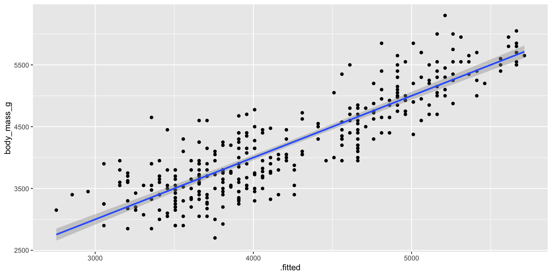

ggplot(a, aes(x = .resid)) +
  geom_histogram()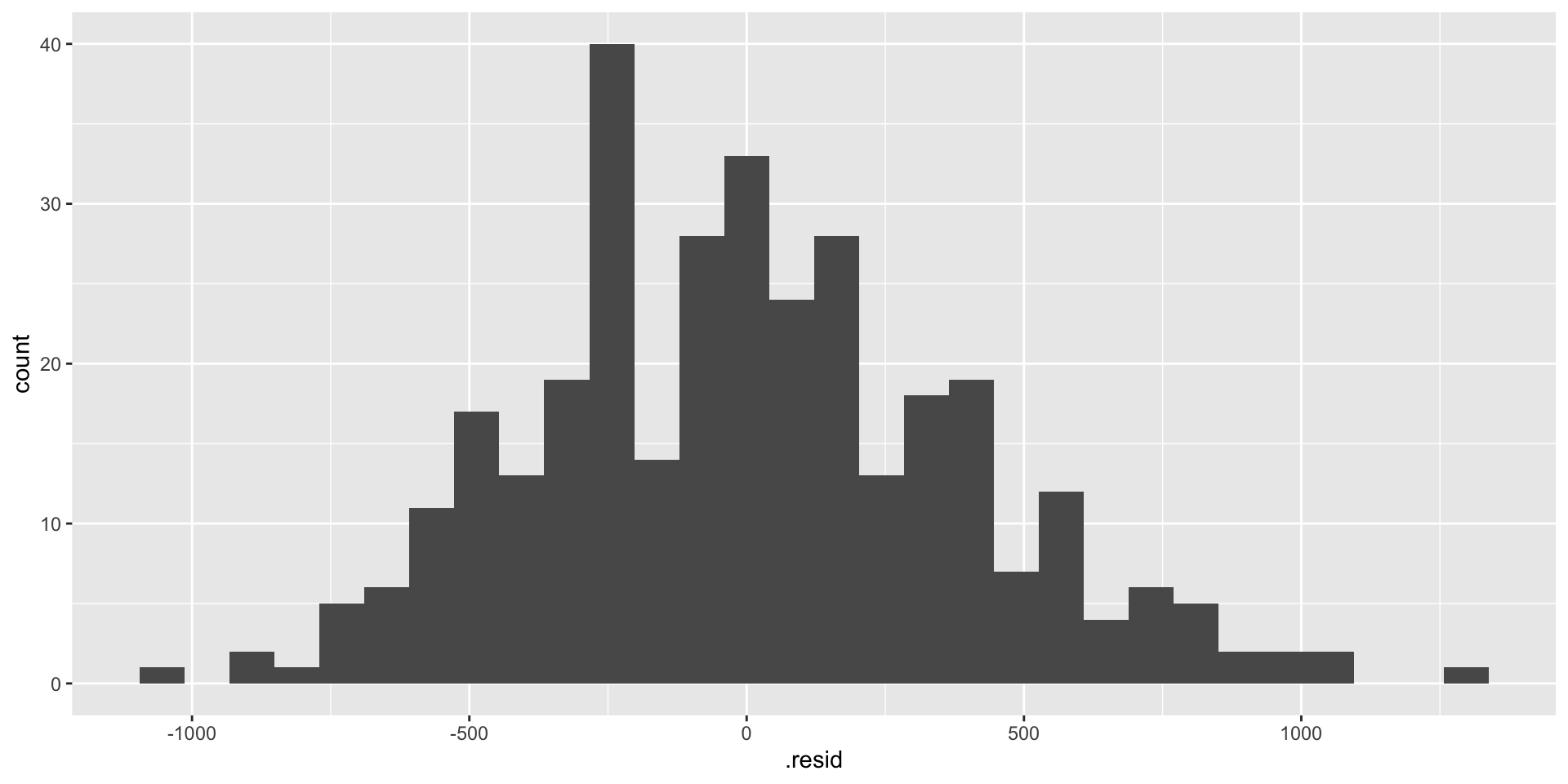

purrr

The purrr package is used for functional programming.
It provides functions for working with lists and vectors.

map

The map() function is used to apply a function to each element of a list.
It is useful when you want to iterate over a list.
Example: Fitting a linear model to each species in the penguins dataset.

penguins |> 
  nest(data = -species) |> 
  mutate(lm = map(data, ~lm(body_mass_g ~ flipper_length_mm, data = .x)))
#> # A tibble: 3 × 3
#>   species   data               lm    
#>   <fct>     <list>             <list>
#> 1 Adelie    <tibble [152 × 7]> <lm>  
#> 2 Gentoo    <tibble [124 × 7]> <lm>  
#> 3 Chinstrap <tibble [68 × 7]>  <lm>

map_*

The map_*() functions are used to extract specific outputs from a list.
They are useful when you want to extract specific outputs from a list.
Example: Extracting the R-squared values (doubles) from the linear models.

penguins |> 
  nest(data = -species) |> 
  mutate(lm = map(data, ~lm(body_mass_g ~ flipper_length_mm, data = .x)),
         r2 = map_dbl(lm, ~summary(.x)$r.squared))
#> # A tibble: 3 × 4
#>   species   data               lm        r2
#>   <fct>     <list>             <list> <dbl>
#> 1 Adelie    <tibble [152 × 7]> <lm>   0.219
#> 2 Gentoo    <tibble [124 × 7]> <lm>   0.494
#> 3 Chinstrap <tibble [68 × 7]>  <lm>   0.412

map2

The map2() function is used to iterate over two lists in parallel.
It is useful when you want to apply a function to two lists simultaneously.
Example: Augmenting the linear models with the original data.

penguins |> 
  drop_na() |> 
  nest(data = -species) |> 
  mutate(lm_mod = map(data, ~lm(body_mass_g ~ flipper_length_mm, data = .x)),
         r2 = map_dbl(lm_mod, ~summary(.x)$r.squared),
         a  = map2(lm_mod, data, ~broom::augment(.x, .y))) 
#> # A tibble: 3 × 5
#>   species   data               lm_mod    r2 a                  
#>   <fct>     <list>             <list> <dbl> <list>             
#> 1 Adelie    <tibble [146 × 7]> <lm>   0.216 <tibble [146 × 13]>
#> 2 Gentoo    <tibble [119 × 7]> <lm>   0.506 <tibble [119 × 13]>
#> 3 Chinstrap <tibble [68 × 7]>  <lm>   0.412 <tibble [68 × 13]>

~ Week 2-3: Spatial Data (Vector)

sf

The sf package is used for working with spatial data.
sf binds to common spatial libraries like GDAL, GEOS, and PROJ.
It provides functions for reading, writing, and manipulating spatial data.

library(sf)

sf::sf_extSoftVersion()
#>           GEOS           GDAL         proj.4 GDAL_with_GEOS     USE_PROJ_H 
#>       "3.11.0"        "3.5.3"        "9.1.0"         "true"         "true" 
#>           PROJ 
#>        "9.1.0"

I/O

The st_read() function is used to read spatial data.
It is useful when you want to import spatial data into R for local or remote files.
Example: Reading a Major Global Rivers.

From package

# via packages
(counties <- AOI::aoi_get(state = "conus", county = "all"))
#> Simple feature collection with 3108 features and 14 fields
#> Geometry type: MULTIPOLYGON
#> Dimension:     XY
#> Bounding box:  xmin: -124.8485 ymin: 24.39631 xmax: -66.88544 ymax: 49.38448
#> Geodetic CRS:  WGS 84
#> First 10 features:
#>    state_region state_division feature_code state_name state_abbr     name
#> 1             3              6      0161526    Alabama         AL  Autauga
#> 2             3              6      0161527    Alabama         AL  Baldwin
#> 3             3              6      0161528    Alabama         AL  Barbour
#> 4             3              6      0161529    Alabama         AL     Bibb
#> 5             3              6      0161530    Alabama         AL   Blount
#> 6             3              6      0161531    Alabama         AL  Bullock
#> 7             3              6      0161532    Alabama         AL   Butler
#> 8             3              6      0161533    Alabama         AL  Calhoun
#> 9             3              6      0161534    Alabama         AL Chambers
#> 10            3              6      0161535    Alabama         AL Cherokee
#>    fip_class tiger_class combined_area_code metropolitan_area_code
#> 1         H1       G4020                388                   <NA>
#> 2         H1       G4020                380                   <NA>
#> 3         H1       G4020                 NA                   <NA>
#> 4         H1       G4020                142                   <NA>
#> 5         H1       G4020                142                   <NA>
#> 6         H1       G4020                 NA                   <NA>
#> 7         H1       G4020                 NA                   <NA>
#> 8         H1       G4020                 NA                   <NA>
#> 9         H1       G4020                122                   <NA>
#> 10        H1       G4020                 NA                   <NA>
#>    functional_status  land_area water_area fip_code
#> 1                  A 1539634184   25674812    01001
#> 2                  A 4117656514 1132955729    01003
#> 3                  A 2292160149   50523213    01005
#> 4                  A 1612188717    9572303    01007
#> 5                  A 1670259090   14860281    01009
#> 6                  A 1613083467    6030667    01011
#> 7                  A 2012002546    2701199    01013
#> 8                  A 1569246126   16536293    01015
#> 9                  A 1545085601   16971700    01017
#> 10                 A 1433620850  120310807    01019
#>                          geometry
#> 1  MULTIPOLYGON (((-86.81491 3...
#> 2  MULTIPOLYGON (((-87.59883 3...
#> 3  MULTIPOLYGON (((-85.41644 3...
#> 4  MULTIPOLYGON (((-87.01916 3...
#> 5  MULTIPOLYGON (((-86.5778 33...
#> 6  MULTIPOLYGON (((-85.65767 3...
#> 7  MULTIPOLYGON (((-86.4482 31...
#> 8  MULTIPOLYGON (((-85.79605 3...
#> 9  MULTIPOLYGON (((-85.59315 3...
#> 10 MULTIPOLYGON (((-85.51361 3...

From file

(rivers <- sf::read_sf('data/majorrivers_0_0/MajorRivers.shp'))
#> Simple feature collection with 98 features and 4 fields
#> Geometry type: MULTILINESTRING
#> Dimension:     XY
#> Bounding box:  xmin: -164.8874 ymin: -36.96945 xmax: 160.7636 ymax: 71.39249
#> Geodetic CRS:  WGS 84
#> # A tibble: 98 × 5
#>    NAME          SYSTEM MILES KILOMETERS                                geometry
#>    <chr>         <chr>  <dbl>      <dbl>                   <MULTILINESTRING [°]>
#>  1 Kolyma        <NA>   2552.      4106. ((144.8419 61.75915, 144.8258 61.8036,…
#>  2 Parana        Parana 1616.      2601. ((-51.0064 -20.07941, -51.02972 -20.22…
#>  3 San Francisco <NA>   1494.      2404. ((-46.43639 -20.25807, -46.49835 -20.2…
#>  4 Japura        Amazon 1223.      1968. ((-76.71056 1.624166, -76.70029 1.6883…
#>  5 Putumayo      Amazon  890.      1432. ((-76.86806 1.300553, -76.86695 1.295,…
#>  6 Rio Maranon   Amazon  889.      1431. ((-73.5079 -4.459834, -73.79197 -4.621…
#>  7 Ucayali       Amazon 1298.      2089. ((-73.5079 -4.459834, -73.51585 -4.506…
#>  8 Guapore       Amazon  394.       634. ((-65.39585 -10.39333, -65.39578 -10.3…
#>  9 Madre de Dios Amazon  568.       914. ((-65.39585 -10.39333, -65.45279 -10.4…
#> 10 Amazon        Amazon 1890.      3042. ((-73.5079 -4.459834, -73.45141 -4.427…
#> # ℹ 88 more rows

via url

# via url
(gage <- sf::read_sf("https://reference.geoconnex.us/collections/gages/items/1000001"))
#> Simple feature collection with 1 feature and 17 fields
#> Geometry type: POINT
#> Dimension:     XY
#> Bounding box:  xmin: -107.2826 ymin: 35.94568 xmax: -107.2826 ymax: 35.94568
#> Geodetic CRS:  WGS 84
#> # A tibble: 1 × 18
#>   nhdpv2_reachcode mainstem_uri           fid nhdpv2_reach_measure cluster uri  
#>   <chr>            <chr>                <int>                <dbl> <chr>   <chr>
#> 1 13020205000216   https://geoconnex.u…     1                 80.3 https:… http…
#> # ℹ 12 more variables: nhdpv2_comid <dbl>, name <chr>, nhdpv2_totdasqkm <dbl>,
#> #   description <chr>, nhdpv2_link_source <chr>, subjectof <chr>,
#> #   nhdpv2_offset_m <dbl>, provider <chr>, gage_totdasqkm <dbl>,
#> #   provider_id <chr>, dasqkm_diff <dbl>, geometry <POINT [°]>

# write out data
# write_sf(counties, "data/counties.shp")

Geometry list columns

The geometry column contains the spatial information.
It is stored as a list-column of sfc objects.
Example: Accessing the first geometry in the rivers dataset.

rivers$geometry[1]
#> Geometry set for 1 feature 
#> Geometry type: MULTILINESTRING
#> Dimension:     XY
#> Bounding box:  xmin: 144.8258 ymin: 61.40833 xmax: 160.7636 ymax: 68.8008
#> Geodetic CRS:  WGS 84

Projections

CRS (Coordinate Reference System) is used to define the spatial reference.
The st_crs() function is used to get the CRS of a dataset.
The st_transform() function is used to transform the CRS of a dataset.
Example: Transforming the rivers dataset to EPSG:5070.

st_crs(rivers) |> sf::st_is_longlat()
#> [1] TRUE
st_crs(rivers)$units
#> NULL

riv_5070  <- st_transform(rivers, 5070)

st_crs(riv_5070) |> sf::st_is_longlat()
#> [1] FALSE

st_crs(riv_5070)$units
#> [1] "m"

Data Manipulation

All dplyr verbs work with sf objects.
Example: Filtering the rivers dataset to include only the Mississippi River.

mississippi <- filter(rivers, SYSTEM == "Mississippi")
larimer     <- filter(counties, name == "Larimer")

Unions / Combines

The st_union() function is used to combine geometries.
It is useful when you want to merge geometries.

mississippi
#> Simple feature collection with 4 features and 4 fields
#> Geometry type: MULTILINESTRING
#> Dimension:     XY
#> Bounding box:  xmin: -112 ymin: 28.92983 xmax: -77.86168 ymax: 48.16158
#> Geodetic CRS:  WGS 84
#> # A tibble: 4 × 5
#>   NAME        SYSTEM      MILES KILOMETERS                              geometry
#> * <chr>       <chr>       <dbl>      <dbl>                 <MULTILINESTRING [°]>
#> 1 Arkansas    Mississippi 1446.      2327. ((-106.3789 39.36165, -106.3295 39.3…
#> 2 Mississippi Mississippi 2385.      3838. ((-95.02364 47.15609, -94.98973 47.3…
#> 3 Missouri    Mississippi 2739.      4408. ((-110.5545 44.76081, -110.6122 44.7…
#> 4 Ohio        Mississippi 1368.      2202. ((-89.12166 36.97756, -89.17502 37.0…

st_union(mississippi)
#> Geometry set for 1 feature 
#> Geometry type: MULTILINESTRING
#> Dimension:     XY
#> Bounding box:  xmin: -112 ymin: 28.92983 xmax: -77.86168 ymax: 48.16158
#> Geodetic CRS:  WGS 84

Measures

The st_length() function is used to calculate the length of a geometry.
The st_area() function is used to calculate the area of a geometry.
The st_distance() function is used to calculate the distance between two geometries.
Example: Calculating the length of the Mississippi River and the area of Larimer County.

st_length(mississippi)
#> Units: [m]
#> [1] 1912869 3147943 3331900 1785519

st_area(larimer)
#> 6813621254 [m^2]

st_distance(larimer, mississippi)
#> Units: [m]
#>          [,1]    [,2]   [,3]    [,4]
#> [1,] 116016.6 1009375 526454 1413983

Predicates

Spatial predicates are used to check relationships between geometries using the DE-9IM model.
The st_intersects() function is used to check if geometries intersect.
The st_filter() function is used to filter geometries based on a predicate.

st_intersects(counties, mississippi)
#> Sparse geometry binary predicate list of length 3108, where the
#> predicate was `intersects'
#> first 10 elements:
#>  1: (empty)
#>  2: (empty)
#>  3: (empty)
#>  4: (empty)
#>  5: (empty)
#>  6: (empty)
#>  7: (empty)
#>  8: (empty)
#>  9: (empty)
#>  10: (empty)

ints <- st_filter(counties, mississippi, .predicate = st_intersects)

ggplot() + 
  geom_sf(data = ints) +
  geom_sf(data = mississippi, col = "blue") + 
  theme_bw()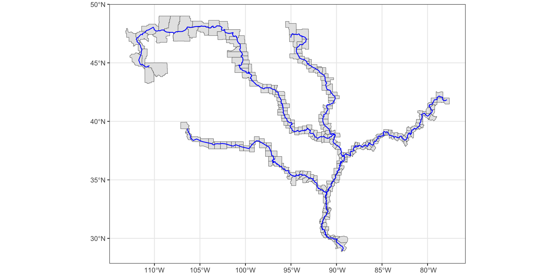

~ Week 4-5: Spatial Data (Raster)

terra

The terra package is used for working with raster data.
It provides functions for reading, writing, and manipulating raster data.

library(terra)
gdal()
#> [1] "3.10.1"

I/O

Any raster format that GDAL can read, can be read with rast().
The package loads the native GDAL src library (like sf)
rast reads data headers, not data itself, until needed.
Example: Reading a GeoTIF of Colorado elevation.

(elev = terra::rast('data/colorado_elevation.tif'))
#> class       : SpatRaster 
#> dimensions  : 16893, 21395, 1  (nrow, ncol, nlyr)
#> resolution  : 30, 30  (x, y)
#> extent      : -1146465, -504615, 1566915, 2073705  (xmin, xmax, ymin, ymax)
#> coord. ref. : +proj=aea +lat_0=23 +lon_0=-96 +lat_1=29.5 +lat_2=45.5 +x_0=0 +y_0=0 +datum=NAD83 +units=m +no_defs 
#> source      : colorado_elevation.tif 
#> name        : CONUS_dem 
#> min value   :     98679 
#> max value   :    439481

Raster Structure

Raster data is stored as an multi-dimensional array of values. - Remember this is atomic vector with diminisions - The same way we looked

v <- values(elev)
head(v)
#>      CONUS_dem
#> [1,]    242037
#> [2,]    243793
#> [3,]    244464
#> [4,]    244302
#> [5,]    244060
#> [6,]    243888
class(v[,1])
#> [1] "integer"

dim(v)
#> [1] 361425735         1
dim(elev)
#> [1] 16893 21395     1
nrow(elev)
#> [1] 16893

Additonal Structure

In addition to the values and diminsions, rasters have: - Extent: The spatial extent of the raster. - Resolution: The spatial resolution of the raster pixels. - CRS: The coordinate reference system of the raster.

crs(elev)
#> [1] "PROJCRS[\"unnamed\",\n    BASEGEOGCRS[\"NAD83\",\n        DATUM[\"North American Datum 1983\",\n            ELLIPSOID[\"GRS 1980\",6378137,298.257222101004,\n                LENGTHUNIT[\"metre\",1]]],\n        PRIMEM[\"Greenwich\",0,\n            ANGLEUNIT[\"degree\",0.0174532925199433]],\n        ID[\"EPSG\",4269]],\n    CONVERSION[\"Albers Equal Area\",\n        METHOD[\"Albers Equal Area\",\n            ID[\"EPSG\",9822]],\n        PARAMETER[\"Latitude of false origin\",23,\n            ANGLEUNIT[\"degree\",0.0174532925199433],\n            ID[\"EPSG\",8821]],\n        PARAMETER[\"Longitude of false origin\",-96,\n            ANGLEUNIT[\"degree\",0.0174532925199433],\n            ID[\"EPSG\",8822]],\n        PARAMETER[\"Latitude of 1st standard parallel\",29.5,\n            ANGLEUNIT[\"degree\",0.0174532925199433],\n            ID[\"EPSG\",8823]],\n        PARAMETER[\"Latitude of 2nd standard parallel\",45.5,\n            ANGLEUNIT[\"degree\",0.0174532925199433],\n            ID[\"EPSG\",8824]],\n        PARAMETER[\"Easting at false origin\",0,\n            LENGTHUNIT[\"metre\",1],\n            ID[\"EPSG\",8826]],\n        PARAMETER[\"Northing at false origin\",0,\n            LENGTHUNIT[\"metre\",1],\n            ID[\"EPSG\",8827]]],\n    CS[Cartesian,2],\n        AXIS[\"easting\",east,\n            ORDER[1],\n            LENGTHUNIT[\"metre\",1,\n                ID[\"EPSG\",9001]]],\n        AXIS[\"northing\",north,\n            ORDER[2],\n            LENGTHUNIT[\"metre\",1,\n                ID[\"EPSG\",9001]]]]"
ext(elev)
#> SpatExtent : -1146465, -504615, 1566915, 2073705 (xmin, xmax, ymin, ymax)
res(elev)
#> [1] 30 30

Crop/Mask

The crop() function is used to crop a raster to a specific extent.
It is useful when you want to work with a subset of the data.
crop extracts data (whether from a remote or local source)
The mask() function is used to mask a raster using a vector or other extent, keeping only the data within the mask.
Input extents must match the CRS of the raster data
Example: Cropping then masking the elevation raster to Larimer County.

larimer_5070 <- st_transform(larimer, crs(elev))

larimer_elev = crop(elev, larimer_5070)

plot(larimer_elev)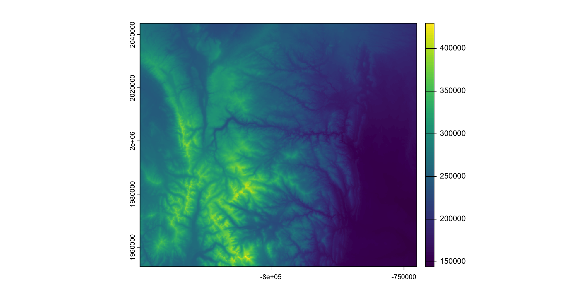

larimer_mask <- mask(larimer_elev, larimer_5070)
plot(larimer_mask)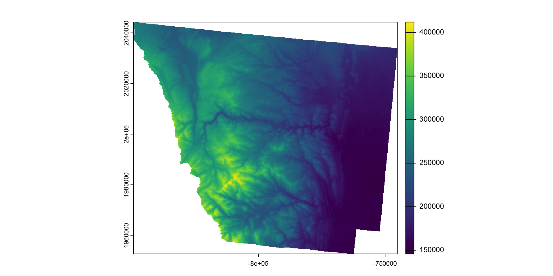

Summary / Algebra

Rasters can be added, subtracted, multiplied, and divided
Any form of map algebra can be done with rasters
For example, multiplying the Larimer mask by 2

raw

larimer_mask
#> class       : SpatRaster 
#> dimensions  : 3054, 3469, 1  (nrow, ncol, nlyr)
#> resolution  : 30, 30  (x, y)
#> extent      : -849255, -745185, 1952655, 2044275  (xmin, xmax, ymin, ymax)
#> coord. ref. : +proj=aea +lat_0=23 +lon_0=-96 +lat_1=29.5 +lat_2=45.5 +x_0=0 +y_0=0 +datum=NAD83 +units=m +no_defs 
#> source(s)   : memory
#> varname     : colorado_elevation 
#> name        : CONUS_dem 
#> min value   :    145787 
#> max value   :    412773

Data Operation

elev2 <- larimer_mask^2

rast modified by rast

larimer_mask / elev2
#> class       : SpatRaster 
#> dimensions  : 3054, 3469, 1  (nrow, ncol, nlyr)
#> resolution  : 30, 30  (x, y)
#> extent      : -849255, -745185, 1952655, 2044275  (xmin, xmax, ymin, ymax)
#> coord. ref. : +proj=aea +lat_0=23 +lon_0=-96 +lat_1=29.5 +lat_2=45.5 +x_0=0 +y_0=0 +datum=NAD83 +units=m +no_defs 
#> source(s)   : memory
#> varname     : colorado_elevation 
#> name        :    CONUS_dem 
#> min value   : 2.422639e-06 
#> max value   : 6.859322e-06

statistical methods

(scaled = scale(larimer_mask))
#> class       : SpatRaster 
#> dimensions  : 3054, 3469, 1  (nrow, ncol, nlyr)
#> resolution  : 30, 30  (x, y)
#> extent      : -849255, -745185, 1952655, 2044275  (xmin, xmax, ymin, ymax)
#> coord. ref. : +proj=aea +lat_0=23 +lon_0=-96 +lat_1=29.5 +lat_2=45.5 +x_0=0 +y_0=0 +datum=NAD83 +units=m +no_defs 
#> source(s)   : memory
#> varname     : colorado_elevation 
#> name        : CONUS_dem 
#> min value   : -1.562331 
#> max value   :  3.053412

Value Supersetting

Rasters are matrices or arrays of values, and can be manipulated as such
For example, setting 35% of the raster to NA

larimer_elev[sample(ncell(larimer_elev), .35*ncell(larimer_elev))] <-  NA

plot(larimer_elev)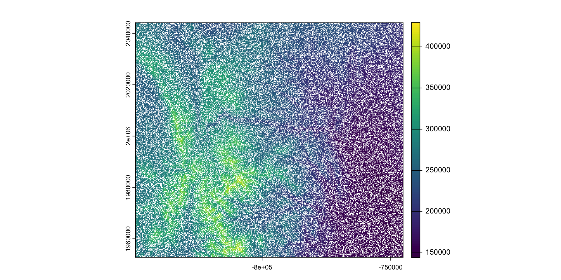

Focal

The focal() function is used to calculate focal statistics.
It is useful when you want to calculate statistics for each cell based on its neighbors.
Example: Calculating the mean elevation within a 30-cell window to remove the NAs we just created

xx = terra::focal(larimer_elev, win = 30, fun  = "mean", na.policy="only")
plot(xx)

~ Week 6-7: Machine Learning

library(tidymodels)
tidymodels_packages()
#>  [1] "broom"        "cli"          "conflicted"   "dials"        "dplyr"       
#>  [6] "ggplot2"      "hardhat"      "infer"        "modeldata"    "parsnip"     
#> [11] "purrr"        "recipes"      "rlang"        "rsample"      "rstudioapi"  
#> [16] "tibble"       "tidyr"        "tune"         "workflows"    "workflowsets"
#> [21] "yardstick"    "tidymodels"

Seeds for reproducability

`rsamples` for resampling and cross-validation

The rsample package is used for resampling and cross-validation.
It provides functions for creating resamples and cross-validation folds.
Example: Creating a 5-fold cross-validation object for the penguins dataset.

set.seed(123)

(penguins_split <- initial_split(drop_na(penguins), prop = 0.8, strata = species))
#> <Training/Testing/Total>
#> <265/68/333>
penguins_train  <- training(penguins_split)
penguins_test   <- testing(penguins_split)

penguin_folds <- vfold_cv(penguins_train, v = 5)

`recipes` for feature engineering

The recipes package is used for feature engineering.
It provides functions for preprocessing data before modeling.
Example: Defining a recipe for feature engineering the penguins dataset.

# Define recipe for feature engineering
penguin_recipe <- recipe(species ~ ., data = penguins_train) |>
  step_impute_knn(all_predictors()) |>         # Impute missing values
  step_normalize(all_numeric_predictors())     # Normalize numeric features

Parsnip for model selection

The parsnip package is used for model implementation
It provides functions for defining models types, engines, and modes.
Example: Defining models for logistic regression, random forest, and decision tree.

# Define models
log_reg_model <- multinom_reg() |> 
  set_engine("nnet")  |> 
  set_mode("classification")

rf_model <- rand_forest(trees = 500) |> 
  set_engine("ranger") |> 
  set_mode("classification")

dt_model <- decision_tree() |> 
  set_mode("classification")

Workflows for model execution

The workflows package is used for model execution.
It provides functions for defining and executing workflows.
Example: Creating a workflow for logistic regression.

# Create workflow
log_reg_workflow <- workflow() |>
  add_model(log_reg_model) |>
  add_recipe(penguin_recipe) |> 
  fit_resamples(resamples = penguin_folds, 
                metrics = metric_set(roc_auc, accuracy))

yardstick for model evaluation

collect_metrics(log_reg_workflow)
#> # A tibble: 2 × 6
#>   .metric  .estimator  mean     n std_err .config             
#>   <chr>    <chr>      <dbl> <int>   <dbl> <chr>               
#> 1 accuracy multiclass     1     5       0 Preprocessor1_Model1
#> 2 roc_auc  hand_till      1     5       0 Preprocessor1_Model1

`workflowsets` for model comparison

The workflowsets package is used for model comparison.
It provides functions for comparing multiple models usingthe purrr mapping paradigm
Example: Comparing logistic regression, random forest, and decision tree models.

(workflowset <- workflow_set(list(penguin_recipe), 
                             list(log_reg_model, rf_model, dt_model)) |> 
  workflow_map("fit_resamples", 
               resamples = penguin_folds, 
               metrics = metric_set(roc_auc, accuracy)))
#> # A workflow set/tibble: 3 × 4
#>   wflow_id             info             option    result   
#>   <chr>                <list>           <list>    <list>   
#> 1 recipe_multinom_reg  <tibble [1 × 4]> <opts[2]> <rsmp[+]>
#> 2 recipe_rand_forest   <tibble [1 × 4]> <opts[2]> <rsmp[+]>
#> 3 recipe_decision_tree <tibble [1 × 4]> <opts[2]> <rsmp[+]>

autoplot / rank_results

The autoplot() function is used to visualize model performance.
The rank_results() function is used to rank models based on a metric.
Example: Visualizing and ranking the model results based on the roc_auc (area under the curve) metric.

autoplot(workflowset)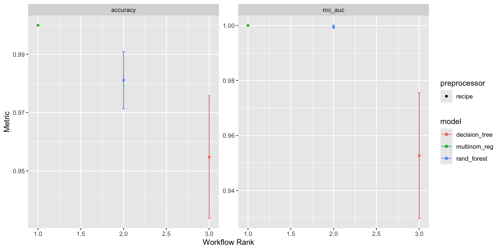

rank_results(workflowset, rank_metric = "roc_auc")
#> # A tibble: 6 × 9
#>   wflow_id          .config .metric  mean std_err     n preprocessor model  rank
#>   <chr>             <chr>   <chr>   <dbl>   <dbl> <int> <chr>        <chr> <int>
#> 1 recipe_multinom_… Prepro… accura… 1     0           5 recipe       mult…     1
#> 2 recipe_multinom_… Prepro… roc_auc 1     0           5 recipe       mult…     1
#> 3 recipe_rand_fore… Prepro… accura… 0.981 5.97e-3     5 recipe       rand…     2
#> 4 recipe_rand_fore… Prepro… roc_auc 1.00  3.60e-4     5 recipe       rand…     2
#> 5 recipe_decision_… Prepro… accura… 0.955 1.28e-2     5 recipe       deci…     3
#> 6 recipe_decision_… Prepro… roc_auc 0.953 1.39e-2     5 recipe       deci…     3

Model Validation

Finally, we can validate the model on the test set
The augment() function is used to add model predictions and residuals to the dataset.
The conf_mat() function is used to create a confusion matrix.
Example: Validating the logistic regression model on the test set.

workflow() |> 
  # Add model and recipe
  add_model(log_reg_model) |>
  add_recipe(penguin_recipe) |>
  # Train model
  fit(data = penguins_train) |> 
  # Fit trained model to test set
  fit(data = penguins_test) |>  
  # Extract Predictions
  augment(penguins_test) |> 
  conf_mat(truth = species, estimate = .pred_class) 
#>            Truth
#> Prediction  Adelie Chinstrap Gentoo
#>   Adelie        30         0      0
#>   Chinstrap      0        14      0
#>   Gentoo         0         0     24

Conclusion

Today we reviewed/introduced the foundations of R for environmental data science.
We discussed data types, structures, and packages for data manipulation and modeling.
We also explored vector and raster data, along with ML applications.
We will continue to build on these concepts in future lectures.
Please complete the survey to help us tailor the course to your needs.

🚀 Getting Started with R for Data Science

Google Survey

~ Week 1: Data Science Basics

Data Types

Data Structures

Vector

Matrix

Array

Data Frame / Tibble

📦 Installing Packages

Attaching/Loading Packages

Help & Documentation

Quarto: Communication

🌟 Tidyverse: A Swiss Army Knife for Data Science R

readr

read_csv

dplyr

%>% / |>

glimpse

select

filter

mutate

summarize

group_by / ungroup

Group operations

Joins

Mutating joins

left_join

right_join

inner_join

full_join

Filtering Joins

ggplot2: Visualization

ggplot

data / aesthetics

geom_*

facet_wrap / facet_grid

theme_*

labs

tidyr

pivot_longer

pivot_wider

nest / unnest

linear modeling: lm

broom

tidy

glance

augment

purrr

map

map_*

map2

~ Week 2-3: Spatial Data (Vector)

sf

I/O

From package

From file

via url

Geometry list columns

Projections

Data Manipulation

Unions / Combines

Measures

Predicates

~ Week 4-5: Spatial Data (Raster)

terra

I/O

Raster Structure

Additonal Structure

Crop/Mask

Summary / Algebra

raw

Data Operation

rast modified by rast

statistical methods

Value Supersetting

Focal

~ Week 6-7: Machine Learning

Seeds for reproducability

rsamples for resampling and cross-validation

`%>%` / `|>`

`ggplot`

`tidyr`

`rsamples` for resampling and cross-validation

`recipes` for feature engineering

`workflowsets` for model comparison