Week 3

Predicates, Simplification & Tesselations

Last week

We learned about the SRS (Spatial Reference Systems)

They can be geographic (3D, angular units)
- Ellipsoid (squished sphere model)
- geoid (mathematical model of gravitational field)
- datum marks the relationship between the ellipsoid and geoid
  - can be local (NAD27)
  - can be global (WGS84, NAD83)
SRS can be projected (x-y axis, measurement units (m), false origin)
- All PCS are based on GCS
- Projections seek to place the 3D earth on 2D
- Does this by defining a plane that can be conic, cylindrical or planar
- “unfolding to this plane” creates distortion of shape, area, distance, or direction
- The distortion is greater from point/lines of tangency or secanacy

Measures (GEOS Measures)

Measures are the questions we ask about the dimension of a geometry
- How long is a line or polygon perimeter (unit)
- What is the area of a polygon (unit²)
- How far are two object from one another (unit)
Measures come from the GEOS library
Measures are in the units of the base projection
Measures can be Euclidean (PCS) or geodesic (GSC)
- geodesic (Great Circle) distances can be more accurate by eliminating distortion
- but are much slower to calculate

For example …

usa <- st_cast(st_union(aoi_get(state = "conus")), "MULTILINESTRING")

nrow(cities)
#> [1] 31254

# Great Circle Distance in GCS
system.time({x <- st_distance(usa, cities)})
# user      system elapsed 
# 103.560   1.390  117.128 

# Euclidean Distance on PCS
system.time({x <- st_distance(usa, cities, which = "Euclidean")})
# user    system  elapsed 
# 2.422   0.019   2.494

Units

When possible measure operations report results with a units appropriate for the CRS:

co <- st_read("data/co.shp")
#> Reading layer `co' from data source 
#>   `/Users/mikejohnson/github/csu-ess-523c/slides/data/co.shp' 
#>   using driver `ESRI Shapefile'
#> Simple feature collection with 64 features and 4 fields
#> Geometry type: MULTIPOLYGON
#> Dimension:     XY
#> Bounding box:  xmin: -109.0602 ymin: 36.99246 xmax: -102.0415 ymax: 41.00342
#> Geodetic CRS:  WGS 84
a <- st_area(co[1,])
attributes(a) |> unlist()
#> units.numerator1 units.numerator2            class 
#>              "m"              "m"          "units"

The units package can be used to convert between units:

units::set_units(a, km^2) # result in square kilometers
#> 3062.85 [km^2]
units::set_units(a, ha) # result in hectares
#> 306285 [ha]

and the results can be stripped of their attributes for cases where numeric values are needed (e.g. math operators and ggplot):

as.numeric(a)
#> [1] 3062849758

Topologic Diminsion

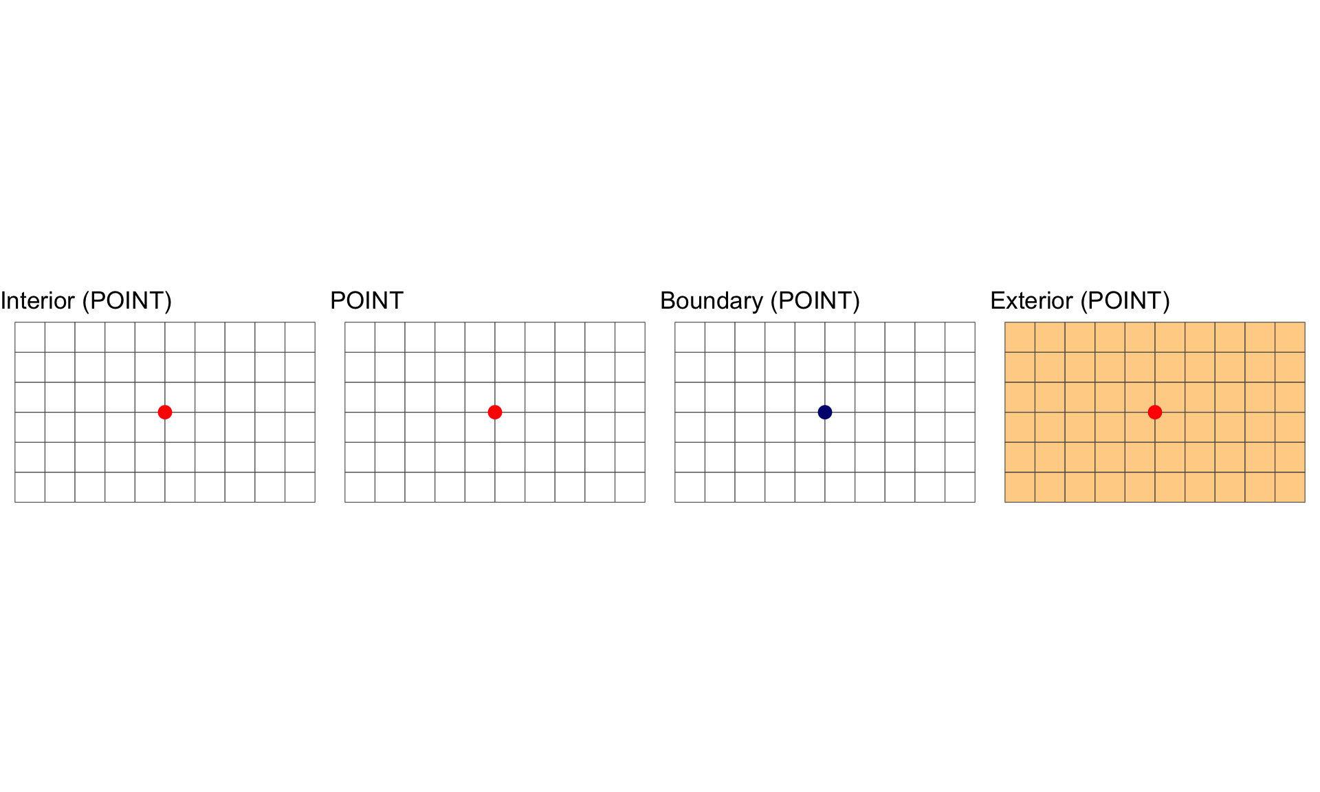
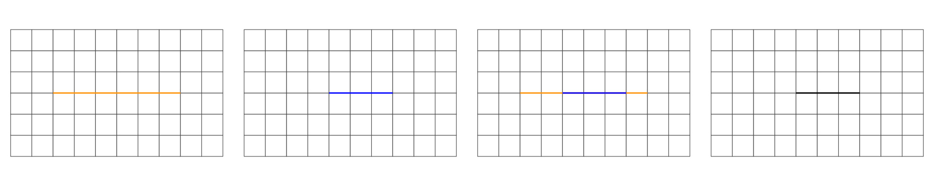
A POINT is shape with a dimension of 0 that occupies a single location in coordinate space.

# POINT defined as numeric vector
(st_dimension(st_point(c(0,1))))
#> [1] 0

A LINESTRING is shape that has a dimension of 1 (length)

# LINESTRING defined by matrix
(st_dimension(st_linestring(matrix(1:4, nrow = 2))))
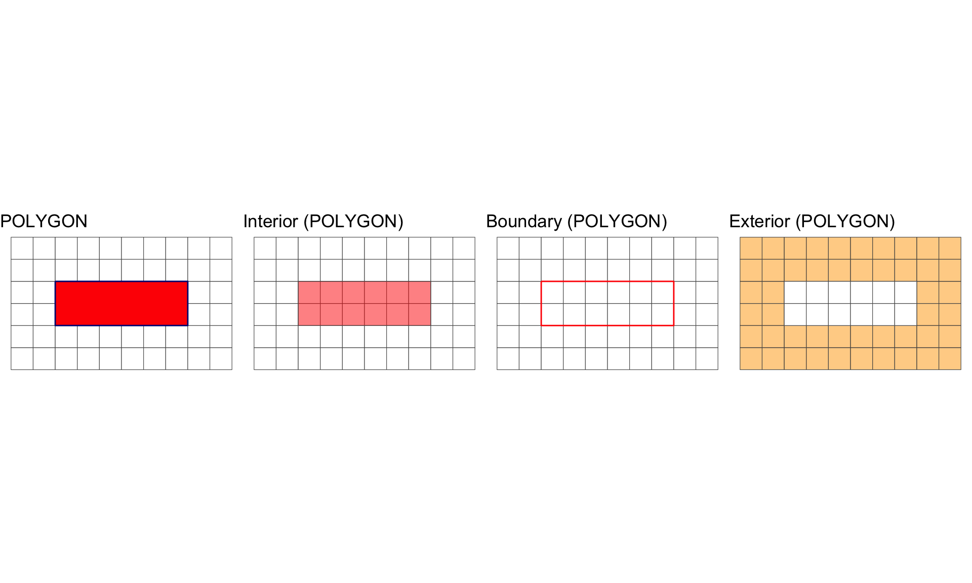
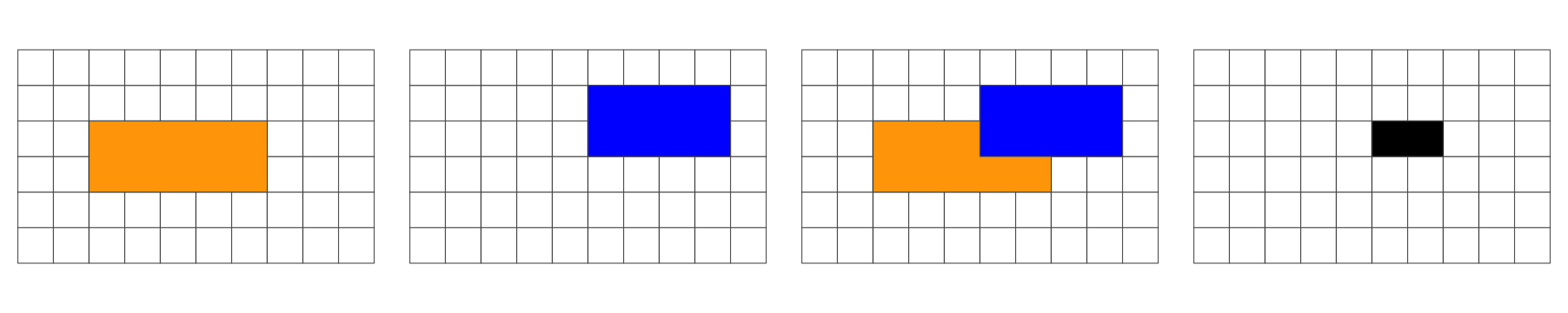
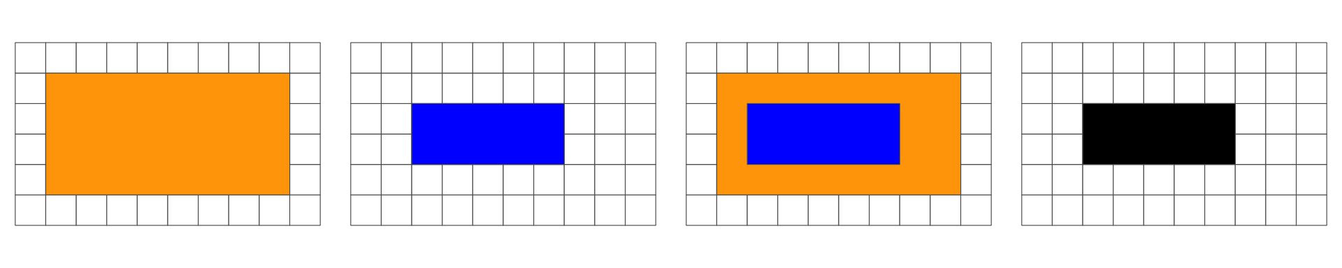
#> [1] 1

A POLYGON is surface stored as a list of its exterior and interior rings. It has a dimension of 2. (area)

# POLYGON defined by LIST (interior and exterior rings)
(st_dimension(st_polygon(list(matrix(c(1:4, 1,2), nrow = 3, byrow = TRUE)))))
#> [1] 2

Predicates

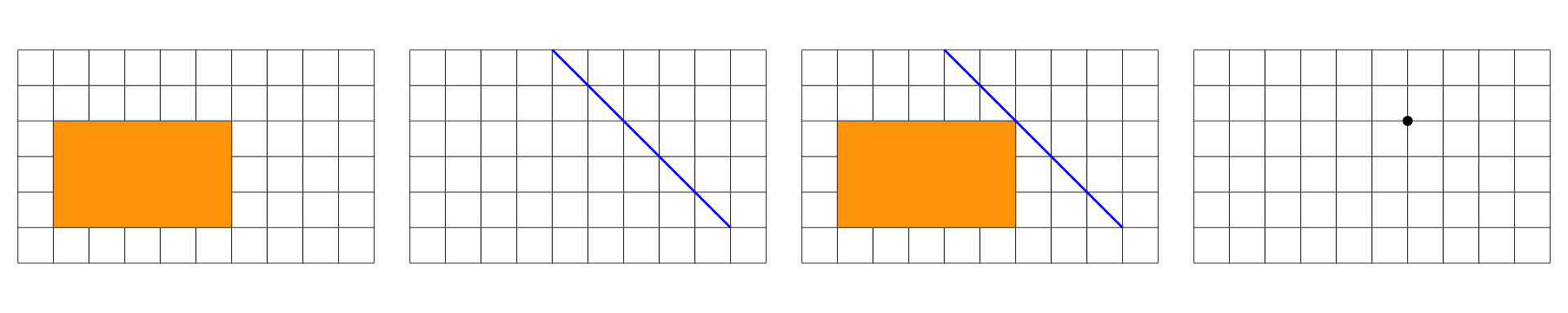
Geometric Interiors, Boundaries and Exteriors

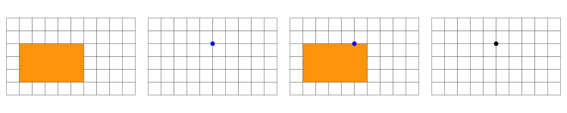
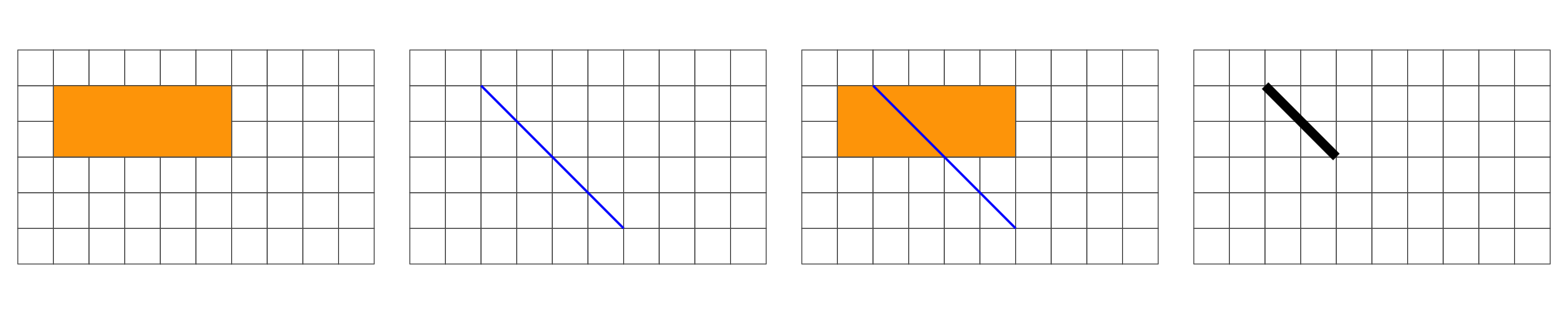
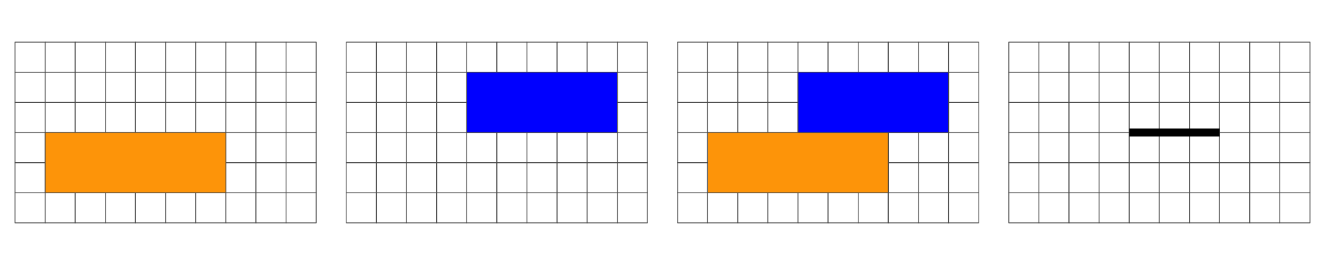
All geometries have interior, boundary and exterior regions.

The terms interior and boundary are used in the context of algebraic topology and manifold theory and not general topology

The OGC has define these states for the common geometry types in the simple features standard:

Dimension	Geometry Type	Interior (I)	Boundary (B)
Point, MultiPoint	0	Point, Points	Empty
LineString, Line	1	Points that are left when the boundary points are removed.	Two end points.
Polygon	2	Points within the rings.	Set of rings.

Interior, Boundary and Exterior: POINTS

Interior, Boundary and Exterior: LINESTRING

#> Warning: Using `size` aesthetic for lines was deprecated in ggplot2 3.4.0.
#> ℹ Please use `linewidth` instead.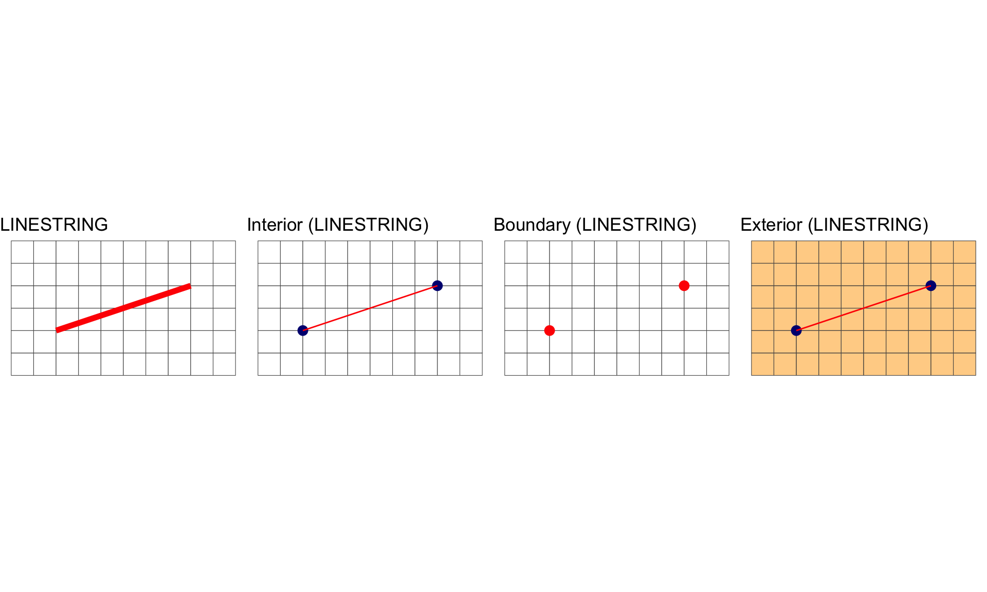

Interior, Boundary and Exterior: POLYGON

Summary

Predicates

In the following, we are interested in the resulting geometry that occurs when 2 geometries are overlaid…

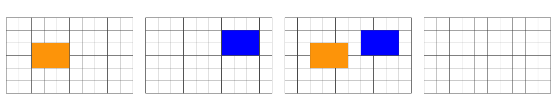
Overlap is a POINT: 0D

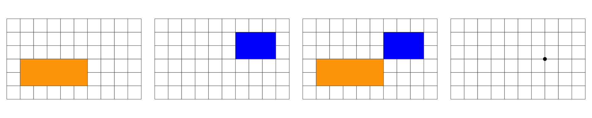
Overlap is a LINESTRING: 1D

Overlap is a POLYGON: 2D

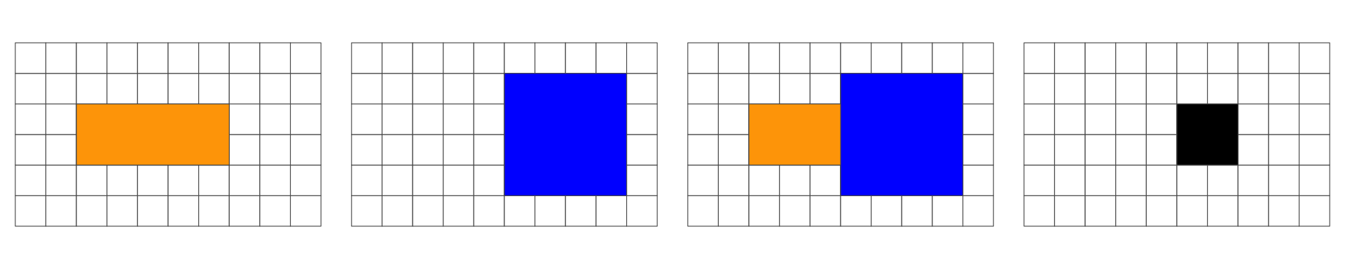
No Overlap = FALSE

Dimensionally Extended 9-Intersection Model

The DE-9IM is a topological model and (standard) used to describe the spatial relations of two geometries
Used in geometry, point-set topology, geospatial topology
The DE-9IM matrix provides a way to classify geometry relations using the set {0,1,2,F} or {T,F}
With a {T,F} matrix domain, there are 512 possible relations that can be grouped into binary classification schemes.
About 10 of these, have been given a common name such as intersects, touches, and within.
When testing two geometries against a scheme, the result is a spatial predicate named by the scheme.
Provides the primary basis for queries and assertions in GIS and spatial databases (PostGIS).

The Matrix Model

The DE-9IM matrix is based on a 3x3 intersection matrix:

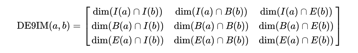
Where:

dim is the dimension of the intersection and
I is the interior
B is the boundary
E is the exterior

. . .

Empty sets are denoted as F

non-empty sets are denoted with the maximum dimension of the intersection {0,1,2}

A simpler (binary) version of this matrix can be created by mapping all non-empty intersections {0,1,2} to TRUE.

Where II would state: “Does the Interior of”a” overlaps with the Interior of “b” in a way that produces a point (0), line (1), or polygon (2)”

Where IB would state: “Does the Interior of”a” overlap with the Boundary of “b” in a way that produces a point (0), line (1), or polygon (2)”

Both matrix forms: - dimensional {0,1,2,F} - Boolean {T,F}

. . .

Can be serialize as a “DE-9IM string code” representing the matrix in a single string element (standardized format for data interchange)

The OGC has standardized the typical spatial predicates (Contains, Crosses, Intersects, Touches, etc.) as Boolean functions, and the DE-9IM model as a function that returns the DE-9IM code, with domain of {0,1,2,F}

Illustration

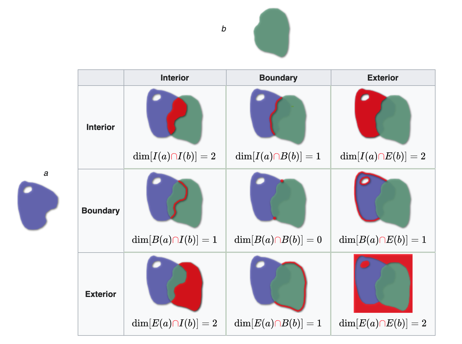
Reading from left-to-right and top-to-bottom, the DE-9IM(a,b) string code is ‘212101212’

Spatial Relations in R

Geometry X is a 3 feature polygon colored in red
Geometry Y is a 4 feature polygon colored in blue

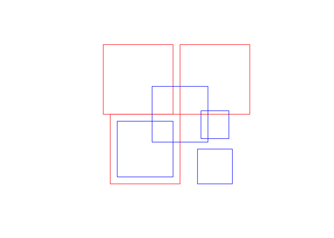
st_relate(x,y)
#>      [,1]        [,2]        [,3]        [,4]       
#> [1,] "212FF1FF2" "FF2FF1212" "212101212" "FF2FF1212"
#> [2,] "FF2FF1212" "212101212" "212101212" "FF2FF1212"
#> [3,] "FF2FF1212" "FF2FF1212" "212101212" "FF2FF1212"
st_relate(x,x)
#>      [,1]        [,2]        [,3]       
#> [1,] "2FFF1FFF2" "FF2F01212" "FF2F11212"
#> [2,] "FF2F01212" "2FFF1FFF2" "FF2FF1212"
#> [3,] "FF2F11212" "FF2FF1212" "2FFF1FFF2"
st_relate(y,y)
#>      [,1]        [,2]        [,3]        [,4]       
#> [1,] "2FFF1FFF2" "FF2FF1212" "212101212" "FF2FF1212"
#> [2,] "FF2FF1212" "2FFF1FFF2" "212101212" "FF2FF1212"
#> [3,] "212101212" "212101212" "2FFF1FFF2" "FF2FF1212"
#> [4,] "FF2FF1212" "FF2FF1212" "FF2FF1212" "2FFF1FFF2"

Named Predicates

“named spatial predicates” have been defined for some common relations.
A few functions can be derived (expressed by masks) from DE-9IM include (* = wildcard):

Predicate	DE-9IM String Code	Description
Intersects	`TFFFF`	“Two geometries intersect if they share any portion of space”
Overlaps	`TFFFF`	“Two geometries overlap if they share some but not all of the same space”
Equals	`TFFFF`	“Two geometries are topologically equal if their interiors intersect and no part of the interior or boundary of one geometry intersects the exterior of the other”
Disjoint	`FFFF****`	“Two geometries are disjoint: they have no point in common. They form a set of disconnected geometries.”
Touches	`FT*******`	`FT***`
Contains	`T***FF`	“A contains B: geometry B lies in A, and the interiors intersect”
Covers	`T****FF`	`T**FF`
Within	`T***FF`	`T*FF`
Covered by	`T***FF`	`T*FF`

Binary Predicates

Collectively, predicates define the type of relationship each 2D object has with another.
Of the ~ 512 unique relationships offered by the DE-9IM models a selection of ~ 10 have been named.
These are include in PostGIS/GEOS and are made accessible via R sf

Named predicates in R

sf provides a set of functions that implement the DE-9IM model and named predicates. Each of these can return either a sparse or dense matrix.

sparse matrix

st_intersects(x,y)
#> Sparse geometry binary predicate list of length 3, where the predicate
#> was `intersects'
#>  1: 1, 3
#>  2: 2, 3
#>  3: 3

dense matrix

st_intersects(x, y, sparse = FALSE)
#>       [,1]  [,2] [,3]  [,4]
#> [1,]  TRUE FALSE TRUE FALSE
#> [2,] FALSE  TRUE TRUE FALSE
#> [3,] FALSE FALSE TRUE FALSE

st_disjoint(x, y, sparse = FALSE)
#>       [,1]  [,2]  [,3] [,4]
#> [1,] FALSE  TRUE FALSE TRUE
#> [2,]  TRUE FALSE FALSE TRUE
#> [3,]  TRUE  TRUE FALSE TRUE

st_touches(x, y, sparse = FALSE)
#>       [,1]  [,2]  [,3]  [,4]
#> [1,] FALSE FALSE FALSE FALSE
#> [2,] FALSE FALSE FALSE FALSE
#> [3,] FALSE FALSE FALSE FALSE

st_within(x, y, sparse = FALSE)
#>       [,1]  [,2]  [,3]  [,4]
#> [1,] FALSE FALSE FALSE FALSE
#> [2,] FALSE FALSE FALSE FALSE
#> [3,] FALSE FALSE FALSE FALSE

st_relates vs. predicate calls…

states = filter(aoi_get(state = "all"), state_abbr %in% c("WA", "OR", "MT", "ID")) |>
  select(name)

wa = filter(states, name == "Washington")

plot(states$geometry)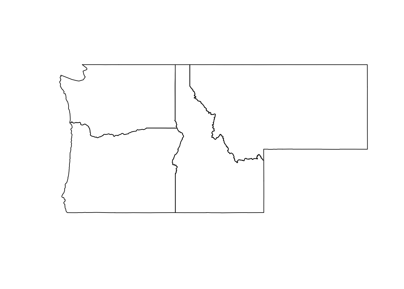

(mutate(states, 
        deim9 = st_relate(states, wa),
        touch = st_touches(states, wa, sparse = F)))
#> Simple feature collection with 4 features and 3 fields
#> Geometry type: MULTIPOLYGON
#> Dimension:     XY
#> Bounding box:  xmin: -124.8485 ymin: 41.98818 xmax: -104.0397 ymax: 49.00244
#> Geodetic CRS:  WGS 84
#>         name                       geometry     deim9 touch
#> 1      Idaho MULTIPOLYGON (((-111.0455 4... FF2F11212  TRUE
#> 2    Montana MULTIPOLYGON (((-109.7985 4... FF2FF1212 FALSE
#> 3     Oregon MULTIPOLYGON (((-117.22 44.... FF2F11212  TRUE
#> 4 Washington MULTIPOLYGON (((-121.5237 4... 2FFF1FFF2 FALSE

So…

binary predicates return conditional {T,F} relations based on predefined masks of the DE-9IM strings
Up to this point in class we have been using Boolean {T,F} masks to filter data.frames by columns:

fruits = c("apple", "orange", "lemon", "watermelon")

fruits == "apple"
#> [1]  TRUE FALSE FALSE FALSE

fruits %in% c("apple", "lemon")
#> [1]  TRUE FALSE  TRUE FALSE

Filtering on data.frames

We have used dplyr::filter to subset a data frame, retaining all rows that satisfy a boolean condition.

mutate(states, equalsWA = (name == "Washington")) |> 
  st_drop_geometry()
#>         name equalsWA
#> 1      Idaho    FALSE
#> 2    Montana    FALSE
#> 3     Oregon    FALSE
#> 4 Washington     TRUE

filter(states, name == "Washington")
#> Simple feature collection with 1 feature and 1 field
#> Geometry type: MULTIPOLYGON
#> Dimension:     XY
#> Bounding box:  xmin: -124.8485 ymin: 45.54364 xmax: -116.9161 ymax: 49.00244
#> Geodetic CRS:  WGS 84
#>         name                       geometry
#> 1 Washington MULTIPOLYGON (((-121.5237 4...

Spatial Filtering

We can filter spatially, use st_filter as the function call
Here the boolean condition is not passed (e.g. name == WA)
But instead, is defined by a spatial predicate
The default is st_intersects but can be changed with the .predicate argument:

mutate(states, 
       touch = st_touches(states, wa, sparse = FALSE)) 
#> Simple feature collection with 4 features and 2 fields
#> Geometry type: MULTIPOLYGON
#> Dimension:     XY
#> Bounding box:  xmin: -124.8485 ymin: 41.98818 xmax: -104.0397 ymax: 49.00244
#> Geodetic CRS:  WGS 84
#>         name                       geometry touch
#> 1      Idaho MULTIPOLYGON (((-111.0455 4...  TRUE
#> 2    Montana MULTIPOLYGON (((-109.7985 4... FALSE
#> 3     Oregon MULTIPOLYGON (((-117.22 44....  TRUE
#> 4 Washington MULTIPOLYGON (((-121.5237 4... FALSE

st_filter(states, wa, .predicate = st_touches) 
#> Simple feature collection with 2 features and 1 field
#> Geometry type: MULTIPOLYGON
#> Dimension:     XY
#> Bounding box:  xmin: -124.7035 ymin: 41.98818 xmax: -111.0435 ymax: 49.00085
#> Geodetic CRS:  WGS 84
#>     name                       geometry
#> 1  Idaho MULTIPOLYGON (((-111.0455 4...
#> 2 Oregon MULTIPOLYGON (((-117.22 44....

Result

ggplot(states) + 
  geom_sf() + 
  geom_sf(data = wa, fill = "blue", alpha = .3) +
  geom_sf(data = st_filter(states, wa, .predicate = st_touches), fill = "red", alpha = .5) + 
  theme_void()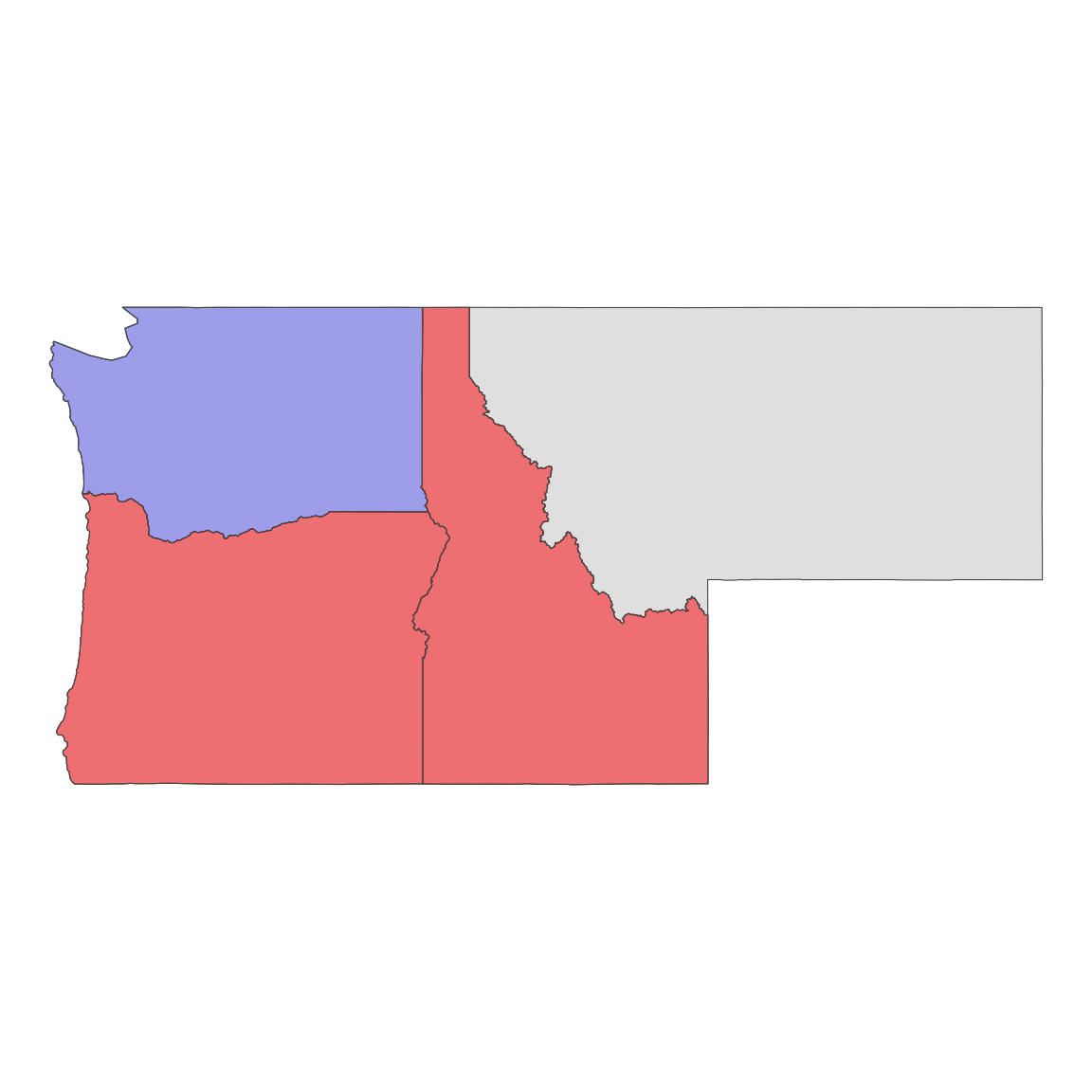

Distance Example (additional parameter)

cities = read_csv("../labs/data/uscities.csv") |> 
  st_as_sf(coords = c("lng", "lat"), crs = 4326) |> 
  select(city, population, state_name) |> 
  st_transform(5070)

st_filter(cities, 
          filter(cities, city == "Fort Collins"), 
          .predicate = st_is_within_distance, 10000) 
#> Simple feature collection with 2 features and 3 fields
#> Geometry type: POINT
#> Dimension:     XY
#> Bounding box:  xmin: -760147.5 ymin: 1982249 xmax: -751658.3 ymax: 1984621
#> Projected CRS: NAD83 / Conus Albers
#> # A tibble: 2 × 4
#>   city         population state_name            geometry
#> * <chr>             <dbl> <chr>              <POINT [m]>
#> 1 Fort Collins     339256 Colorado   (-760147.5 1984621)
#> 2 Timnath            8007 Colorado   (-751658.3 1982249)

Spatial Data Science

Filtering is a nice way to reduce the dimensions of a single dataset
Often “… one table is not enough… ”
In these cases we want to combine - or join - data

Spatial Joining

Joining two non-spatial datasets relies on a shared key that uniquely identifies each record in a table

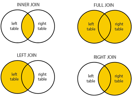
Spatially joining data relies on shared geographic relations rather then a shared key
Like filter, these relations can be defined by a predicate
As with tabular data, mutating joins add data to the target object (x) from a source object (y).

st_join

In sf st_join provides this joining capacity
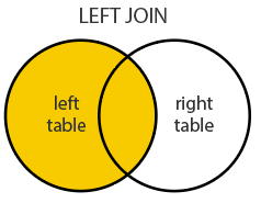
By default, st_join performs a left join (Returns all records from x, and the matched records from y)

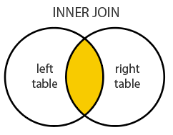
It can also do inner joins by setting left = FALSE.

The default predicate for st_join (and st_filter) is st_intersects
This can be changed with the join argument (see ?st_join for details).

Every Starbucks in the World

What county has the most Starbucks in each state?

(starbucks = readr::read_csv('../labs/data/directory.csv') |> 
  filter(!is.na(Latitude), Country == "US") |> 
  st_as_sf(coords = c("Longitude", "Latitude"), crs = 4326) |> 
  st_transform(5070))
#> Simple feature collection with 13608 features and 11 fields
#> Geometry type: POINT
#> Dimension:     XY
#> Bounding box:  xmin: -6223543 ymin: 278590.9 xmax: 2122577 ymax: 5307178
#> Projected CRS: NAD83 / Conus Albers
#> # A tibble: 13,608 × 12
#>    Brand     `Store Number` `Store Name` `Ownership Type` `Street Address` City 
#>  * <chr>     <chr>          <chr>        <chr>            <chr>            <chr>
#>  1 Starbucks 3513-125945    Safeway-Anc… Licensed         5600 Debarr Rd … Anch…
#>  2 Starbucks 74352-84449    Safeway-Anc… Licensed         1725 Abbott Rd   Anch…
#>  3 Starbucks 12449-152385   Safeway - A… Licensed         1501 Huffman Rd  Anch…
#>  4 Starbucks 24936-233524   100th & C S… Company Owned    320 W. 100th Av… Anch…
#>  5 Starbucks 8973-85630     Old Seward … Company Owned    1005 E Dimond B… Anch…
#>  6 Starbucks 72788-84447    Fred Meyer … Licensed         1000 E Northern… Anch…
#>  7 Starbucks 79549-106150   Safeway - A… Licensed         3101 PENLAND PK… Anch…
#>  8 Starbucks 75988-107245   ANC Main Te… Licensed         HMSHost, 500 We… Anch…
#>  9 Starbucks 11426-99254    Tudor Rd an… Company Owned    110 W. Tudor Rd… Anch…
#> 10 Starbucks 20349-108249   Fred Meyer-… Licensed         7701 Debarr Road Anch…
#> # ℹ 13,598 more rows
#> # ℹ 6 more variables: `State/Province` <chr>, Country <chr>, Postcode <chr>,
#> #   `Phone Number` <chr>, Timezone <chr>, geometry <POINT [m]>

counties = aoi_get(state = "conus", county = "all") |> 
  st_transform(5070) |> 
  select(name, state_name)

topSB <- st_join(counties, starbucks) |> 
  group_by(name, state_name) |> 
  summarise(n = n()) |> 
  group_by(state_name) |> 
  slice_max(n, n = 1) |> 
  ungroup()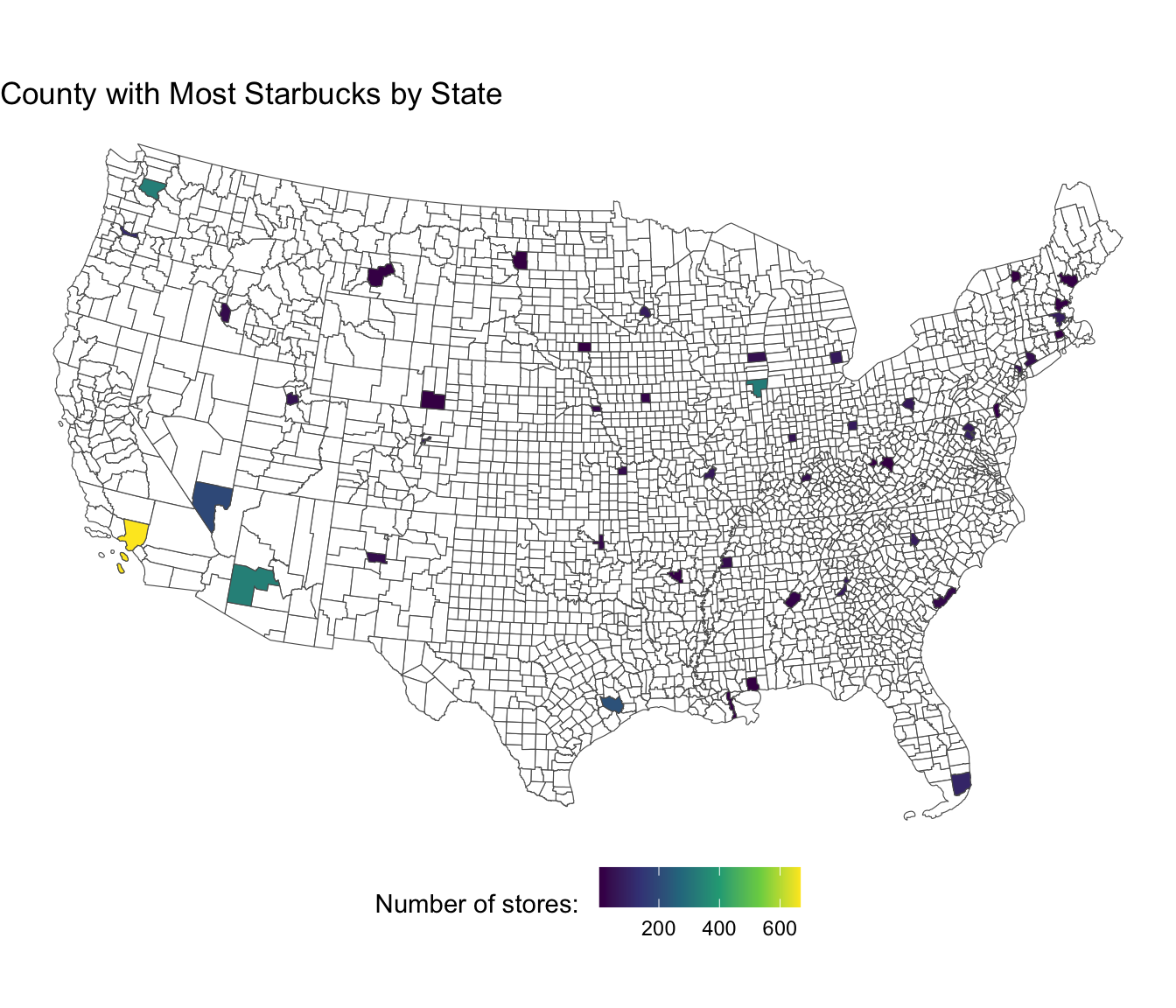

Neither joining nor filtering spatially alter the underlying geometry of the features
In cases where we seek to alter a geometry based on another, we need clipping methods

Clipping

Clipping is a form of subsetting that involves changing the geometry of at least some features.
Clipping can only apply to features more complex than points: (lines, polygons and their ‘multi’ equivalents).

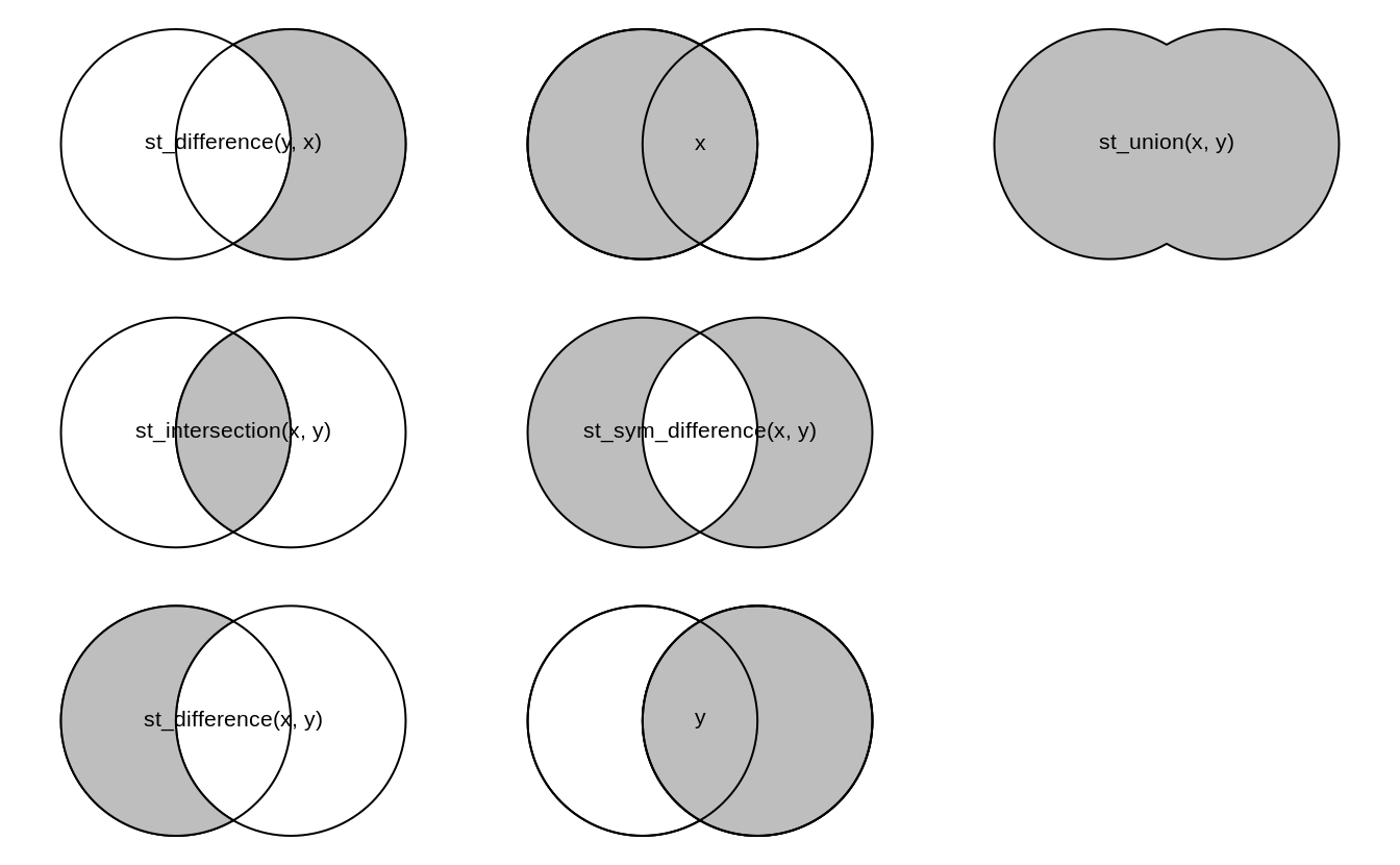
Spatial Subsetting

By default the data.frame subsetting methods we’ve seen (e.g [,]) implements st_intersection

wa = st_transform(wa, 5070)
wa_starbucks = starbucks[wa,] #<<

ggplot() + geom_sf(data = wa) + geom_sf(data = wa_starbucks) + theme_void()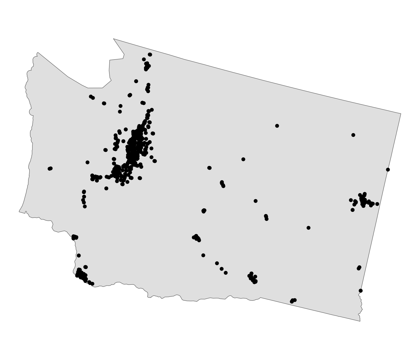

Simplification

Computational Complexity

In all the cases we have looked at, the number of POINT (e.g geometries, nodes, or vertices) define the complexity of the predicate or the clip
Computational needs increase with the number of POINTS / NODES / VERTICES
Simplification is a process for generalization vector objects (lines and polygons)
Another reason for simplifying objects is to reduce the amount of memory, disk space and network bandwidth they consume
Other times the level of detail captured in a geometry is either not needed, or, even counter productive the the scale/purpose of an analysis
If you are cropping features to a national border, how much detail do you need? The more points in your border, the long the clip operation will take….

In cases where we want to reduce the complexity in a geometry we can use simplification algorithms

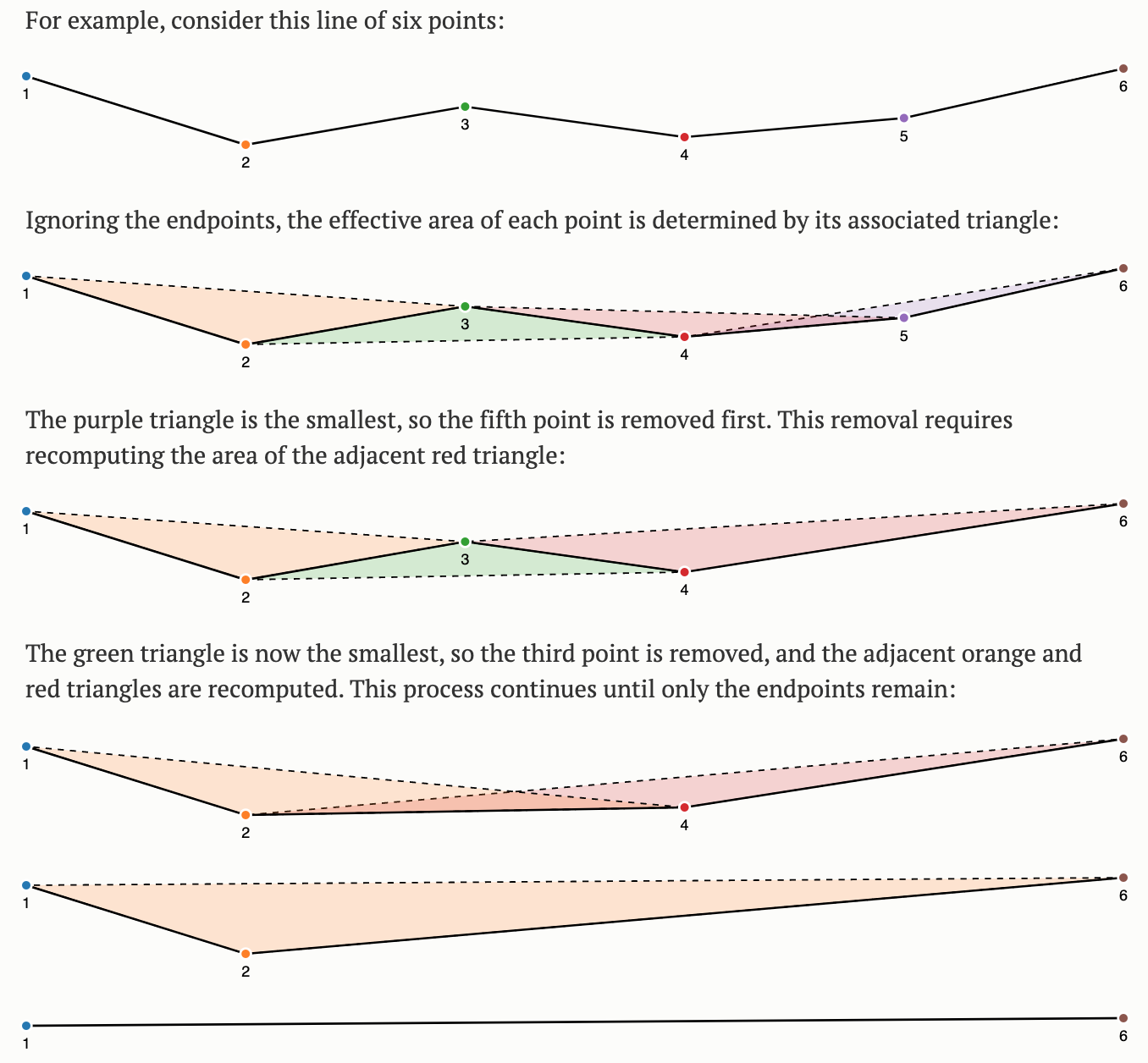
The most common algorithms are Ramer–Douglas–Peucker and Visvalingam-Whyatt.

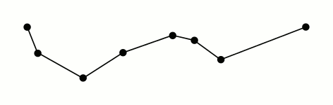
Ramer–Douglas–Peucker

Mark the first and last points as kept
Find the point, p that is the farthest from the first-last line segment. If there are no points between first and last we are done (the base case)
If p is closer than tolerance units to the line segment then everything between first and last can be discarded
Otherwise, mark p as kept and repeat steps 1-4 using the points between first and p and between p and last (the call to recursion)

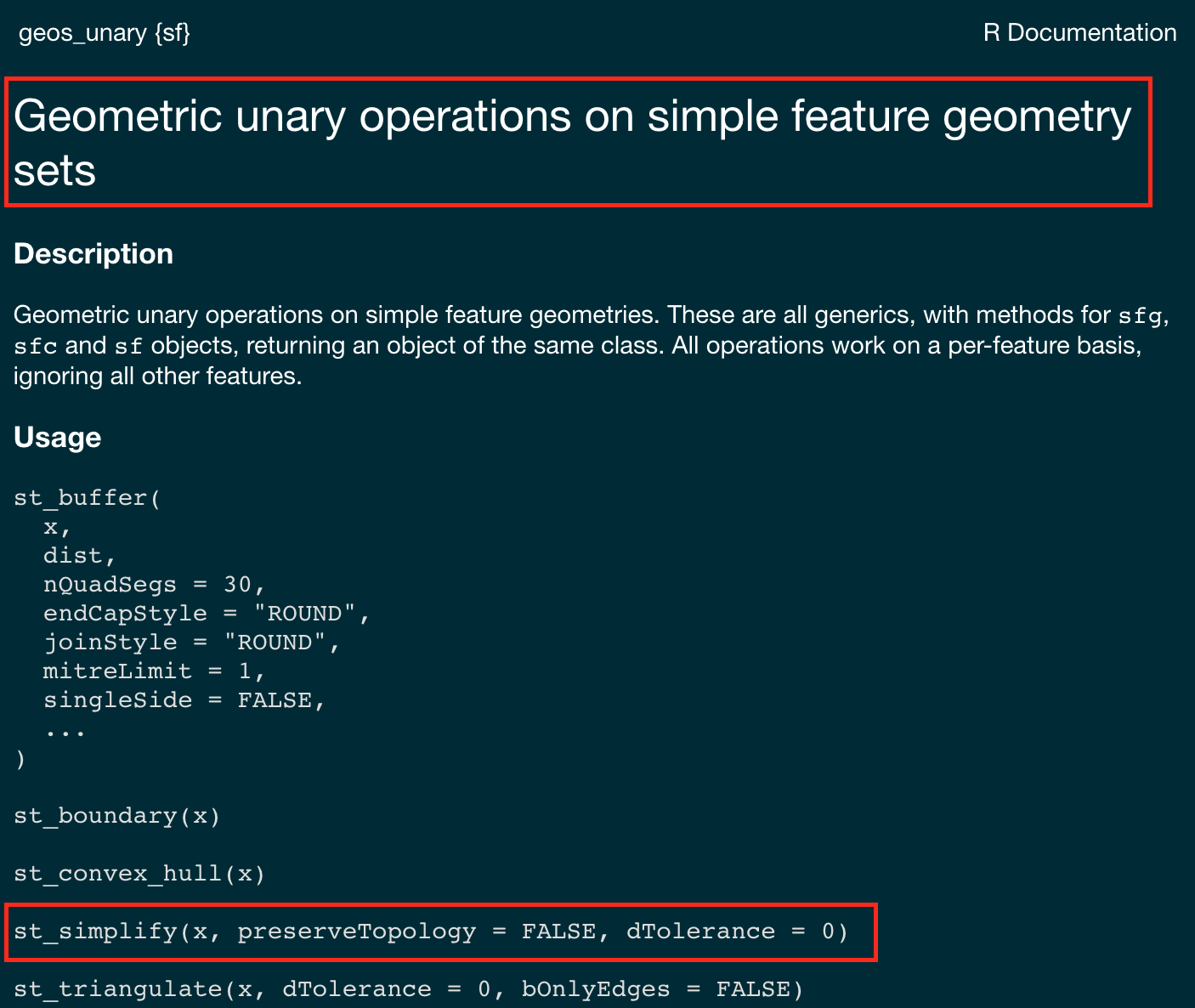
st_simplify

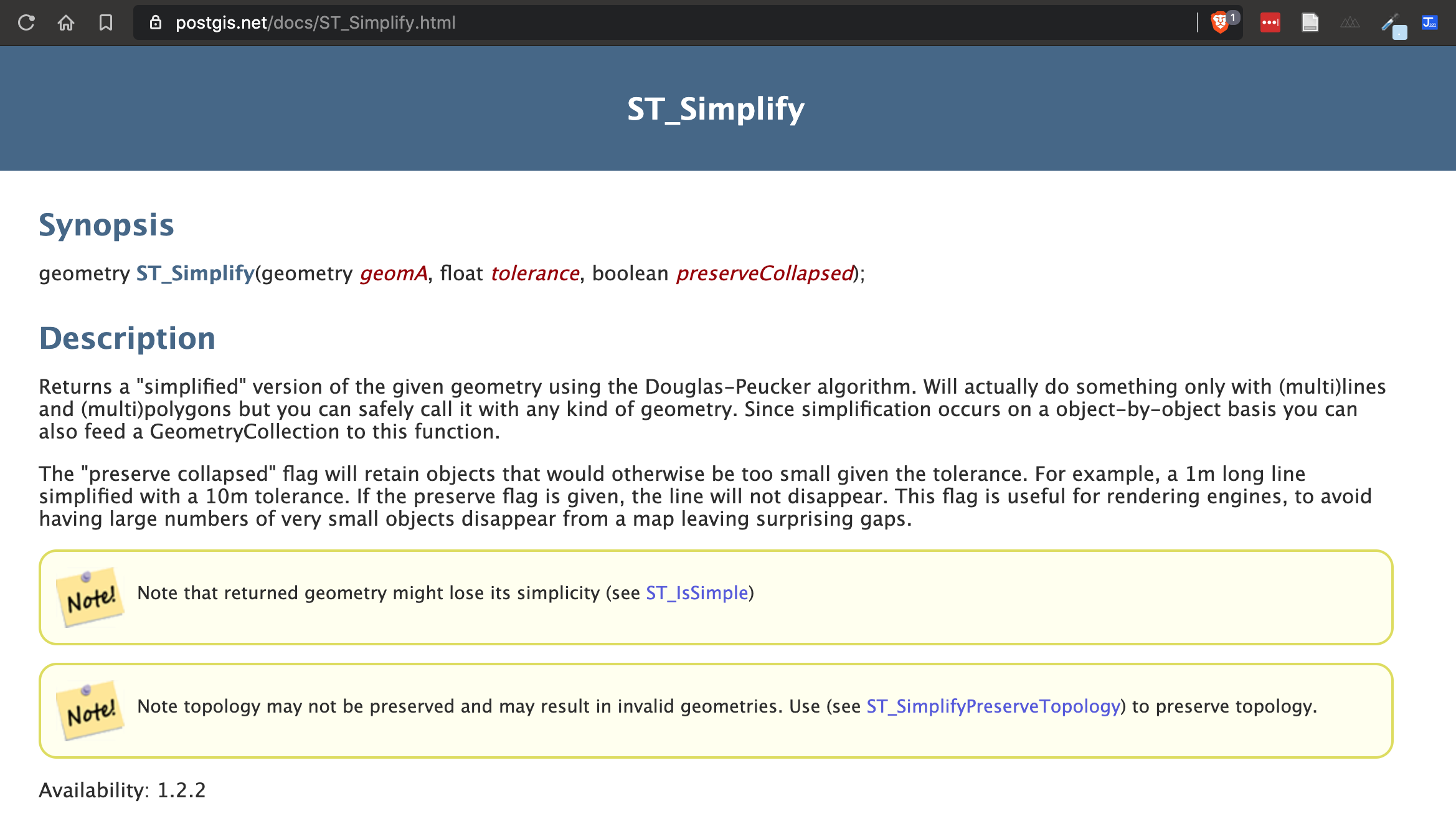
st_simplify

sf provides st_simplify, which uses the GEOS implementation of the Douglas-Peucker algorithm to reduce the vertex count.
st_simplify uses the dTolerance to control the level of generalization in map units (see Douglas and Peucker 1973 for details).

usa = aoi_get(state = "conus") |> 
  st_union() |> 
  st_transform(5070)

usa1000   = st_simplify(usa, dTolerance = 10000)
usa10000  = st_simplify(usa, dTolerance = 100000)
usa100000 = st_simplify(usa, dTolerance = 1000000)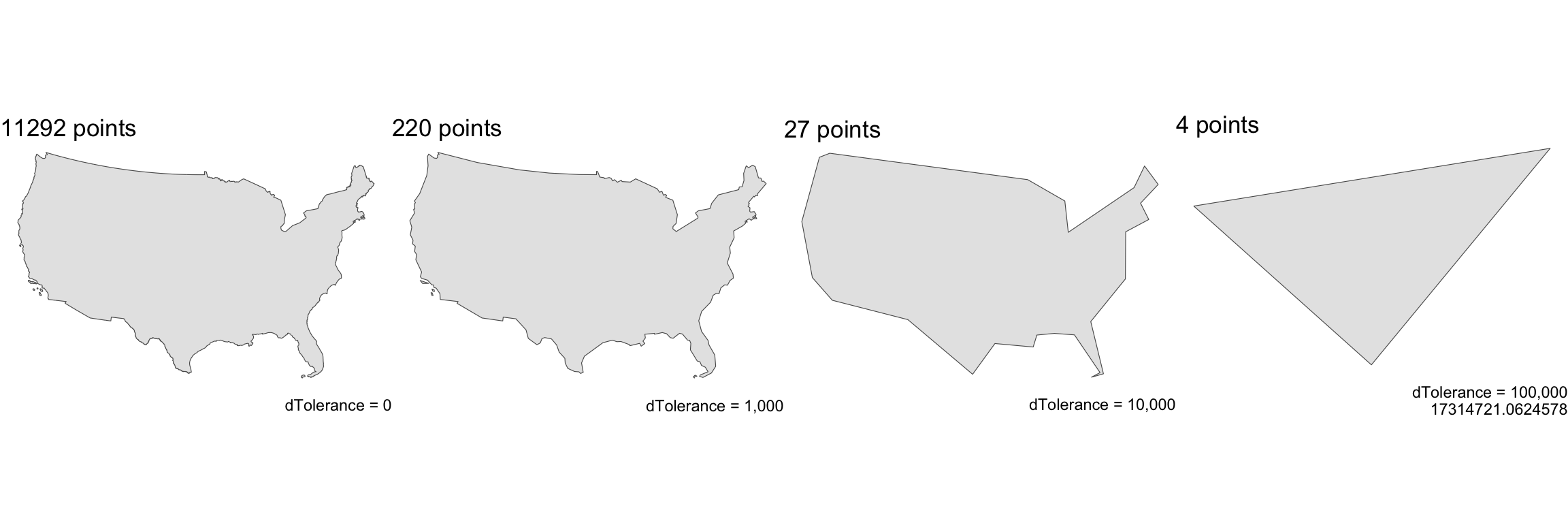

A limitation with Douglas-Peucker (therefore st_simplify) is that it simplifies objects on a per-geometry basis.
This means the ‘topology’ is lost, resulting in overlapping and disconnected geometries.

states = st_transform(states, 5070)
simp_states   = st_simplify(states, dTolerance = 20000)
plot(simp_states$geometry)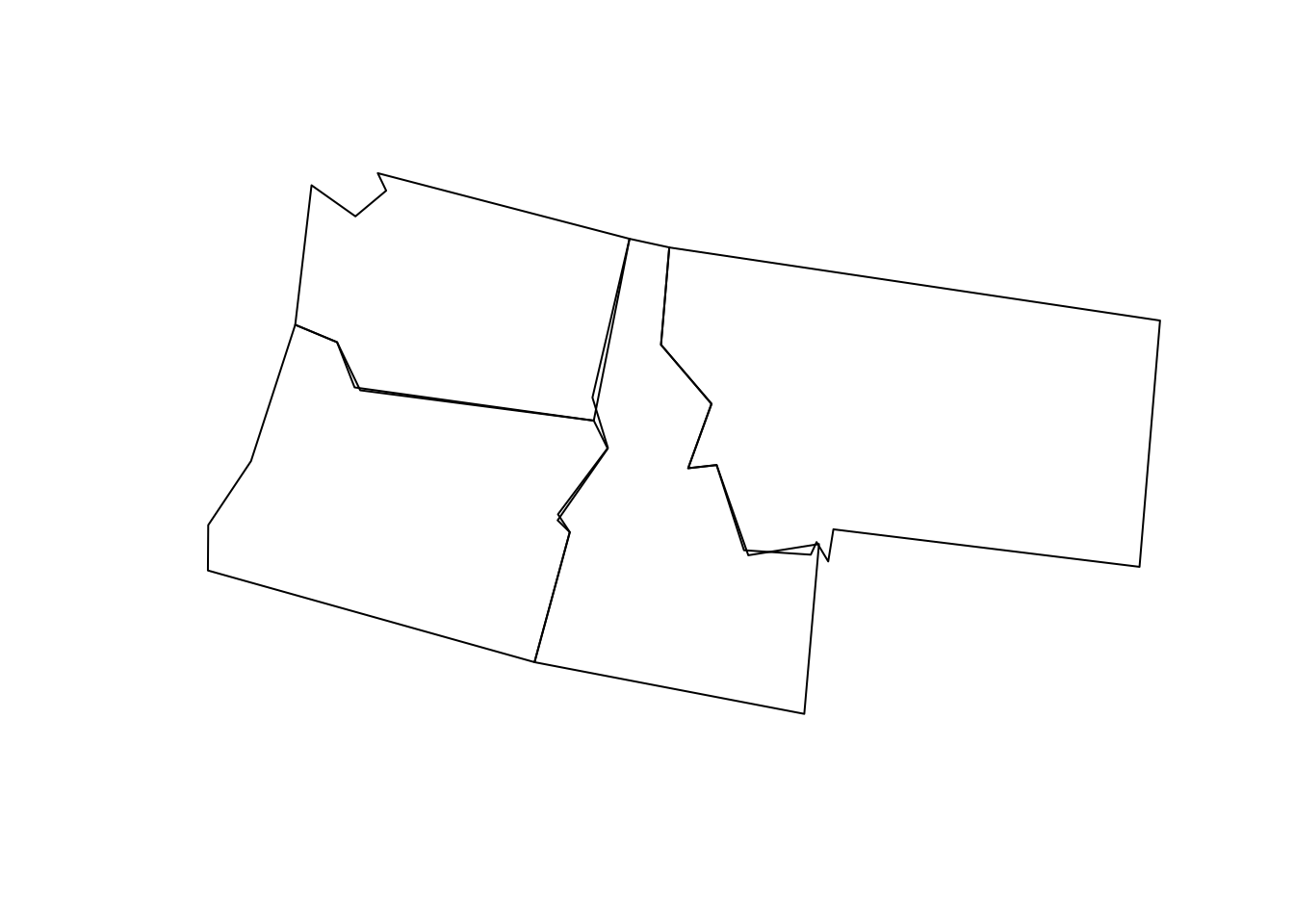

Visvalingam

The Visvalingam algorithm overcomes some limitations of the Douglas-Peucker algorithm (Visvalingam and Whyatt 1993).
it progressively removes points with the least-perceptible change.
Simplification often allows the elimination of 95% or more points while retaining sufficient detail for visualization and often analysis

rmapshaper

In R, the rmapshaper package implements the Visvalingam algorithm in the ms_simplify function.

The ms_simplify function is a wrapper around the mapshaper JavaScript library (created by lead viz experts at the NYT)

library(rmapshaper)

usa10 = ms_simplify(usa, keep = .1)
usa5  = ms_simplify(usa, keep = .05)
usa1  = ms_simplify(usa, keep = .01)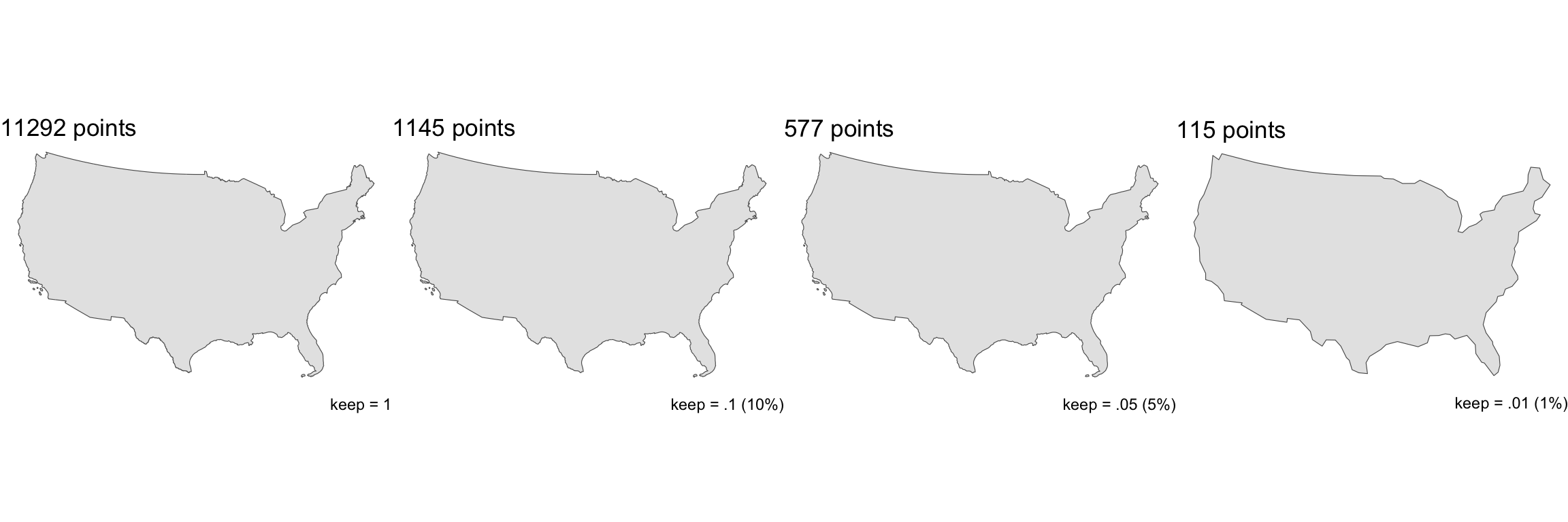

states = st_transform(states, 5070)
simp_states   = ms_simplify(states, keep = .05)
plot(simp_states$geometry)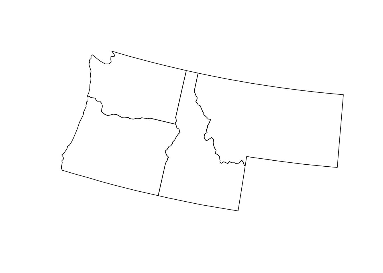

In all cases, the number of points in a geometry can be calculated with mapview::npts()

states = st_transform(states, 5070)
simp_states_st   = st_simplify(states, dTolerance = 20000)
simp_states_ms   = ms_simplify(states, keep = .05)

mapview::npts(states)
#> [1] 5930
mapview::npts(simp_states_st)
#> [1] 50
mapview::npts(simp_states_ms)
#> [1] 292

Tesselation

So far we have spent the last few days looking at simple feature objects
Where a feature as a geometry define by a set of structured POINT(s)
These points have precision and define location ({X Y CRS})
The geometry defines a bounds: either 0D, 1D or 2D
Each object is therefore bounded to those geometries implying a level of exactness.

Core Concepts of Spatial Data: (Kuhn 2012)

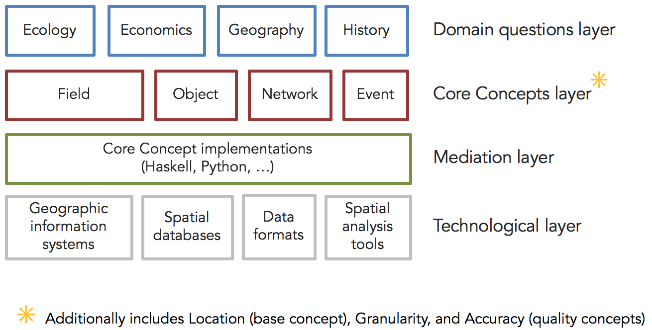
Core Concepts of Spatial Data: (Kuhn 2012)

One Base Concept: Location
Four Content Concepts: Field, Object, Network, Event
Two Quality Concepts: Granularity, Accuracy

Core Concepts of Spatial Data: (Kuhn 2012)

One Base Concept: Location (coordinates)
Four Content Concepts: Field (raster), Object (simple feature), ~~Network~~, ~~Event~~
Two Quality Concepts: Granularity (simplification), Accuracy (taken for granted)

Object View

Objects describe individuals that have an identity (id) as well as spatial, temporal, and thematic properties.
Answers questions about properties and relations of objects.
Results from fixing theme, controlling time, and measuring space.
Features, such as surfaces, depend on objects (but are also objects)

Object View

Object implies boundedness
- boundaries may not be known or even knowable, but have limits.
Crude examples of such limits are the minimal bounding boxes used for indexing and querying objects in databases.
Many objects (particularly natural ones) do not have crisp boundaries (watersheds)
Differences between spatial information from multiple sources are often caused by more or less arbitrary delineations through context-dependent boundaries.
Many questions about objects and features can be answered without boundaries, using simple point representations (centroids) with thematic attributes.

Field View

Fields describe phenomena that have a scalar or vector attribute everywhere in a space of interest
- for example, air temperatures, rainfall, elevation, land cover
Field information answers the question what is here?, where here can be anywhere in the space considered.
Field-based spatial information can also represent attributes that are computed rather than measured, such as probabilities or densities.

Together, fields and objects are the two fundamental ways of structuring spatial information.

Objects can provide coverage:

Both objects and fields can cover space continuously - the primary difference is that objects prescribe bounds.
- Counties are one form of object that covers the USA seamlessly
- State objects are another …

Object Coverages

LANDSAT Path Row

Serves tiles based on a path/row index

#> Warning in layer_sf(geom = GeomSf, data = data, mapping = mapping, stat = stat,
#> : Ignoring unknown aesthetics: label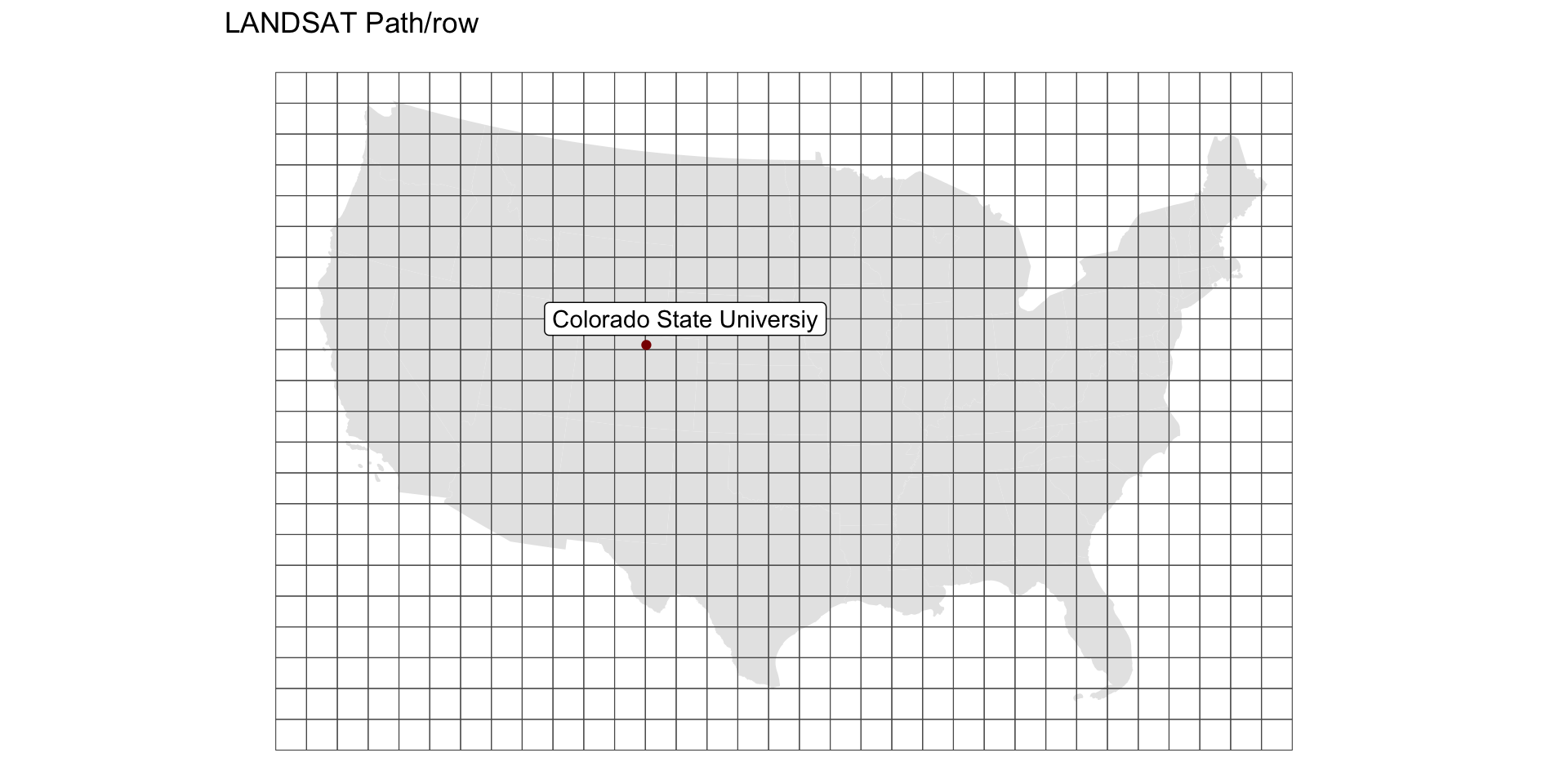

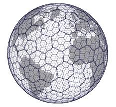
MODIS Sinisoial Grid

Serves tiles based on a path/row index

#> Warning: st_crs<- : replacing crs does not reproject data; use st_transform for
#> that
#> Warning in layer_sf(geom = GeomSf, data = data, mapping = mapping, stat = stat,
#> : Ignoring unknown aesthetics: label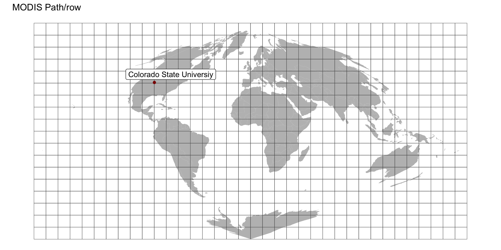

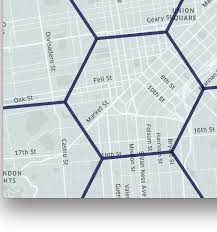
Uber Hex Addressing

Breaks the world into Hexagons…

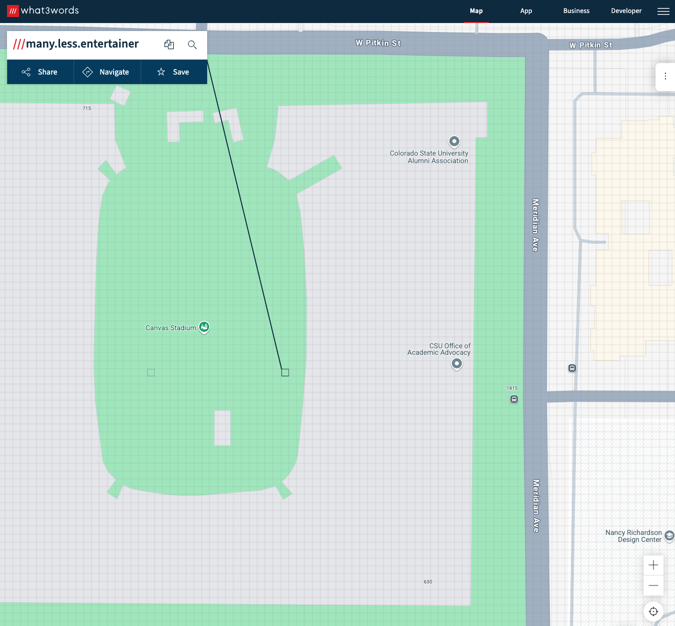
what3word

Breaks the world into 3m grids encoded with unique 3 word strings

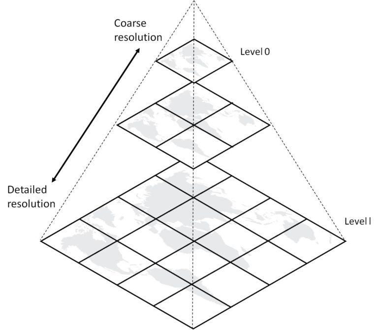
Map Tiles / slippy maps / Pyramids

Use XYZ where Z is a zoom level …

Our Data for today …

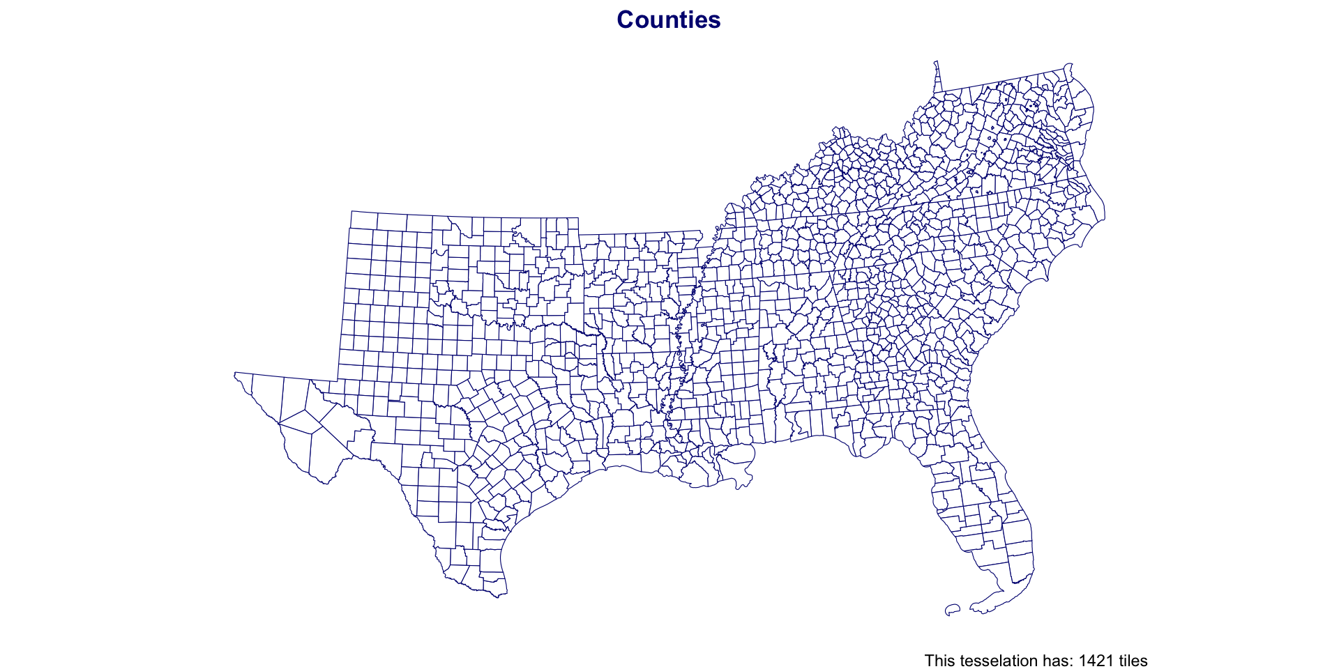
Southern Counties

south_counties = aoi_get(state = "south", county = "all") |> 
  st_transform(st_crs(cities))

Unioned to States using `dplyr`

south_states = south_counties |> 
  group_by(state_name) |> 
  summarise()

South County Centroids

south_cent = st_centroid(south_counties)
#> Warning: st_centroid assumes attributes are constant over geometries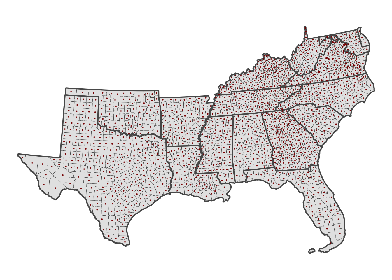

Southern Coverage: County

Regular Tiles

One way to tile a surface is into regions of equal area
Tiles can be either square (rectilinear) or hexagonal
st_make_grid generates a square or hexagonal grid covering the geometry of an sf or sfc object
The return object of st_make_grid is a new sfc object
Grids can be specified by cellsize or number of grid cells (n) in the X and Y direction

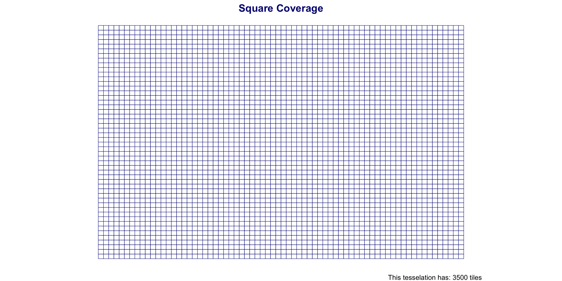
# Create a grid over the south with 70 rows and 50 columns
sq_grid = st_make_grid(south_counties, n = c(70, 50)) |> 
  st_as_sf() |> 
  mutate(id = 1:n())

Southern Coverage: Square

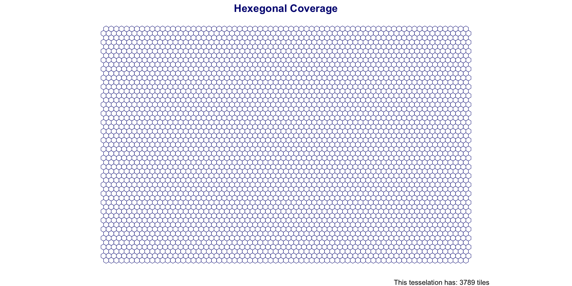
Hexagonal Grid

Hexagonal tessellations (honey combs) offer an alternative to square grids
They are created in the same way but by setting square = FALSE

hex_grid = st_make_grid(south_counties, n = c(70, 50), square = FALSE) |> 
  st_as_sf() |> 
  mutate(id = 1:n())

Southern Coverage: Hexagon

Advantages Square Grids

Simple definition and data storage
- Only need the origin (lower left), cell size (XY) and grid dimensions
Easy to aggregate and dissaggregate (resample)
Analogous to raster data
Relationship between cells is given
Combining layers is easy with traditional matrix algebra

Advantages Square Grids

Reduced Edge Effects
- Lower perimeter to area ratio
- minimizes the amount line length needed to create a lattice of cells with a given area
All neighbors are identical
- No rook vs queen neighbors
Better fit to curve surfaces (e.g. the earth)

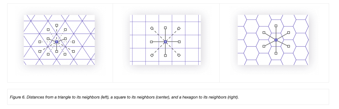
Triangulations

An alternative to creating equal area tiles is to create triangulations from known anchor points
Triangulation requires a set of input points and seeks to partition the interior into a partition of triangles.
In GIS contexts you’ll hear:
- Thiessen Polygon
- Voronoi Regions
- Delunay Triangulation
- TIN (Triangular irregular networks)
- etc,..

Voronoi Polygons

Voronoi/Thiessen polygon boundaries define the area closest to each anchor point relative to all others
They are defined by the perpendicular bisectors of the lines between all points.

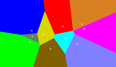
Voronoi Polygons

Voronoi Polygons

Usefull for tasks such as:
- nearest neighbor search,
- facility location (optimization),
- largest empty areas,
- path planning…
Also useful for simple interpolation of values such as rain gauges,

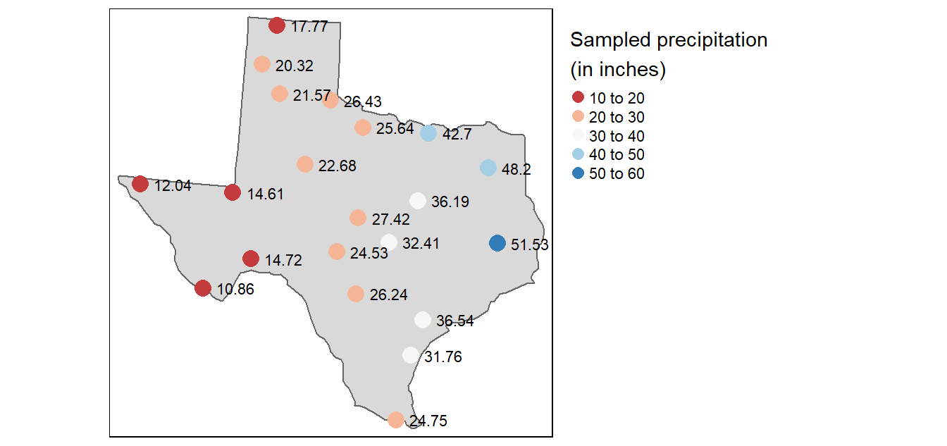
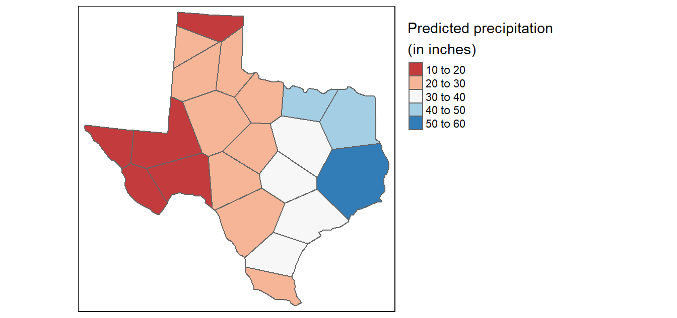
Often used in numerical models and simulations

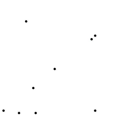
`st_voronoi`

st_voronoi creates voronoi tesselation in sf
It works over a MULTIPOINT collection
Should always be simplified after creation (st_cast())
If to be treated as an object for analysis, should be id’d

south_cent_u = st_union(south_cent)

v_grid = st_voronoi(south_cent_u) |> 
  st_cast() |> 
  st_as_sf() |> 
  mutate(id = 1:n())

Southern Coverage: Voronoi

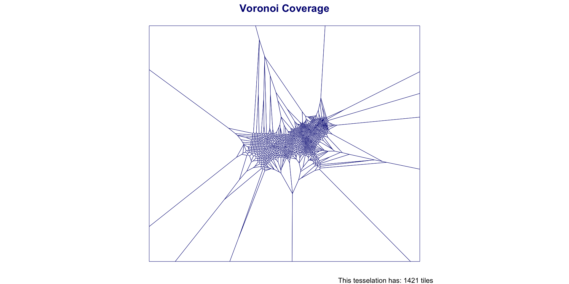
Southern Coverage: Voronoi

#> Warning: attribute variables are assumed to be spatially constant throughout
#> all geometries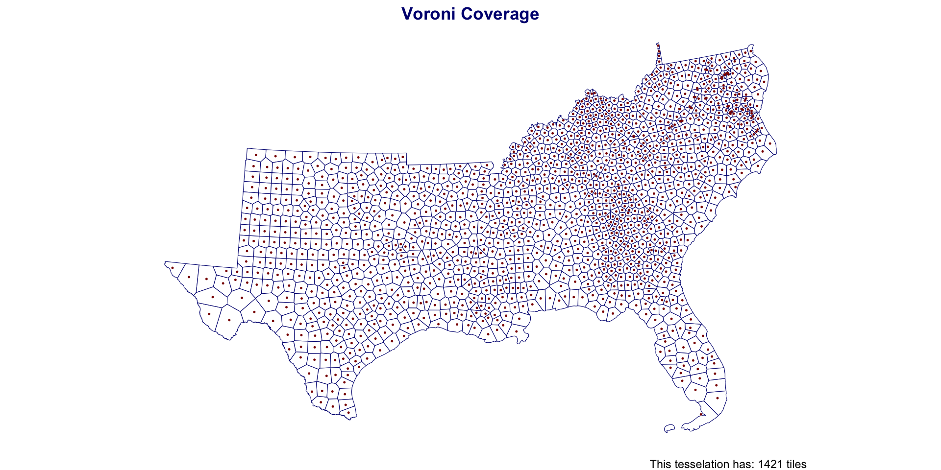

Delaunay triangulation

A Delaunay triangulation for a given set of points (P) in a plane, is a triangulation DT(P), where no point is inside the circumcircle of any triangle in DT(P).

Delaunay triangulation

The Delaunay triangulation of a discrete POINT set corresponds to the dual graph of the Voronoi diagram.
The circumcenters (center of circles) of Delaunay triangles are the vertices of the Voronoi diagram.

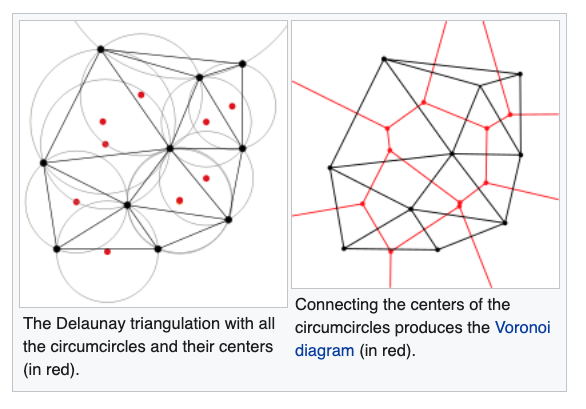
Used in landscape evaluation and terrian modeling

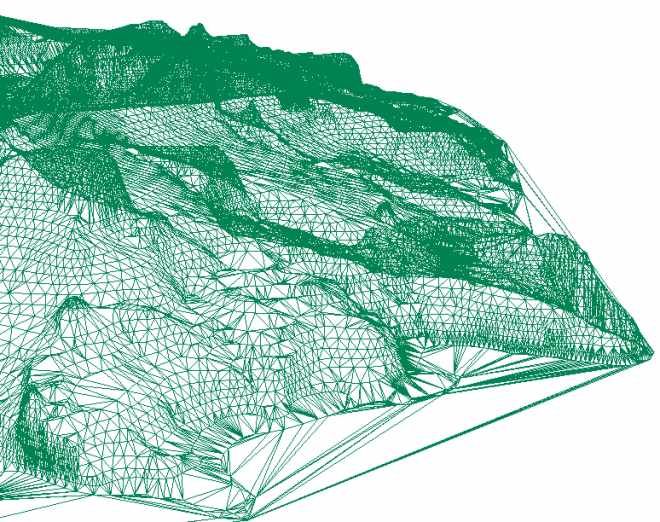
`st_triangulate`

st_triangulate creates Delaunay triangulation in sf
It works over a MULTIPOINT collection
Should always be simplified after creation (st_cast())
If to be treated as an object for analysis, should be id’d

t_grid = st_triangulate(south_cent_u) |> 
  st_cast() |> 
  st_as_sf() |> 
  mutate(id = 1:n())

Southern Coverage: Triangles

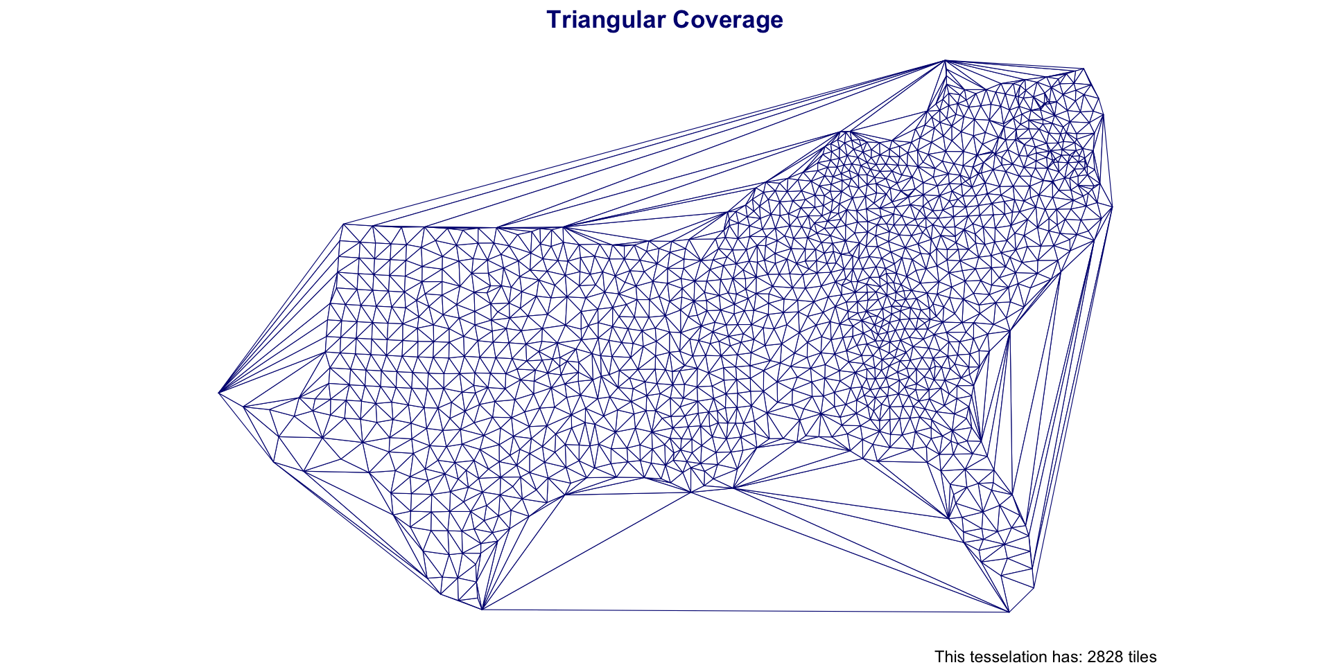
Southern Coverage: Triangles

t_grid = st_intersection(t_grid, st_union(south_states))
#> Warning: attribute variables are assumed to be spatially constant throughout
#> all geometries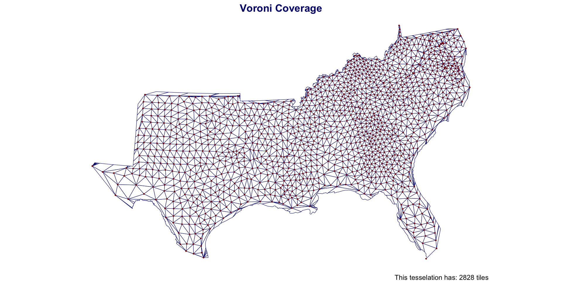

Difference in object coverages:

Tesselation Characteristics
Type	Elements	Mean Area (km2)	Standard Deviation Area (km2)	Coverage Area
triangulation	2,828	832	557	2,352,288
voroni	1,421	1,688	1,046	2,398,383
counties	1,421	1,688	1,216	2,398,383
grid	3,500	1,470	0	5,144,369
Hexagon	3,789	1,425	0	5,398,416

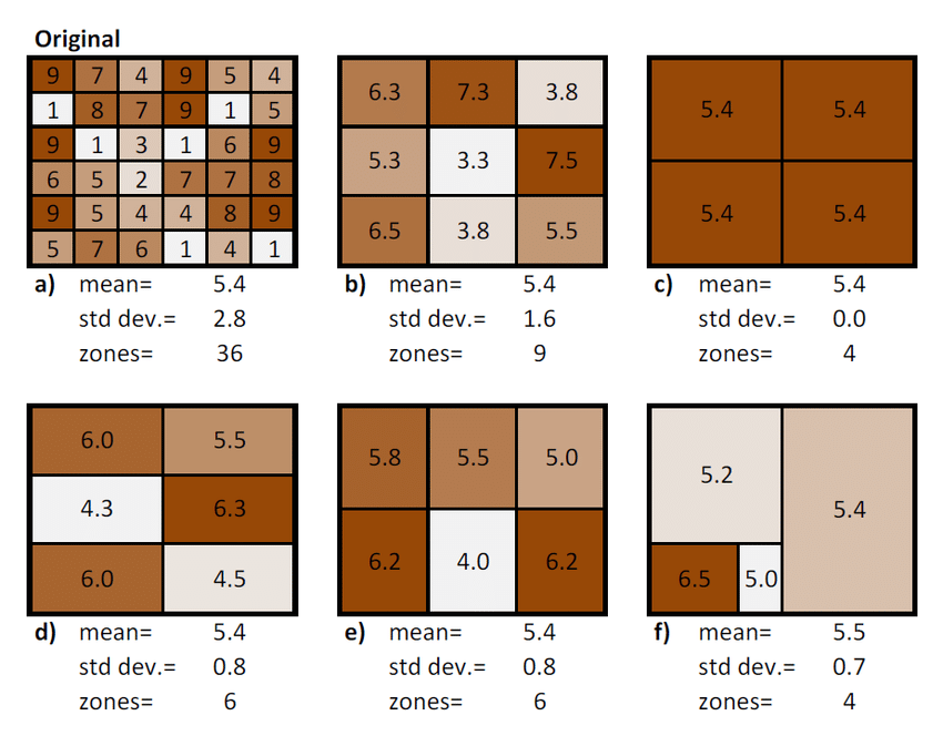
Modifiable areal unit problem (MAUP)

The modifiable areal unit problem (MAUP) is a source of statistical bias that can significantly impact the results of statistical hypothesis tests.
MAUP affects results when point-based measures are aggregated into districts.
The resulting summary values (e.g., totals or proportions) are influenced by both the shape and scale of the aggregation unit.

Real World Example

The power of GIS is the ability to integrate different layers and types of information
The scale of information can impact the analysis as can the grouping and zoning schemes chosen
The Modifiable Areal Unit Problem (MAUP) is an important issue for those who conduct spatial analysis using units of analysis at aggregations higher than incident level.
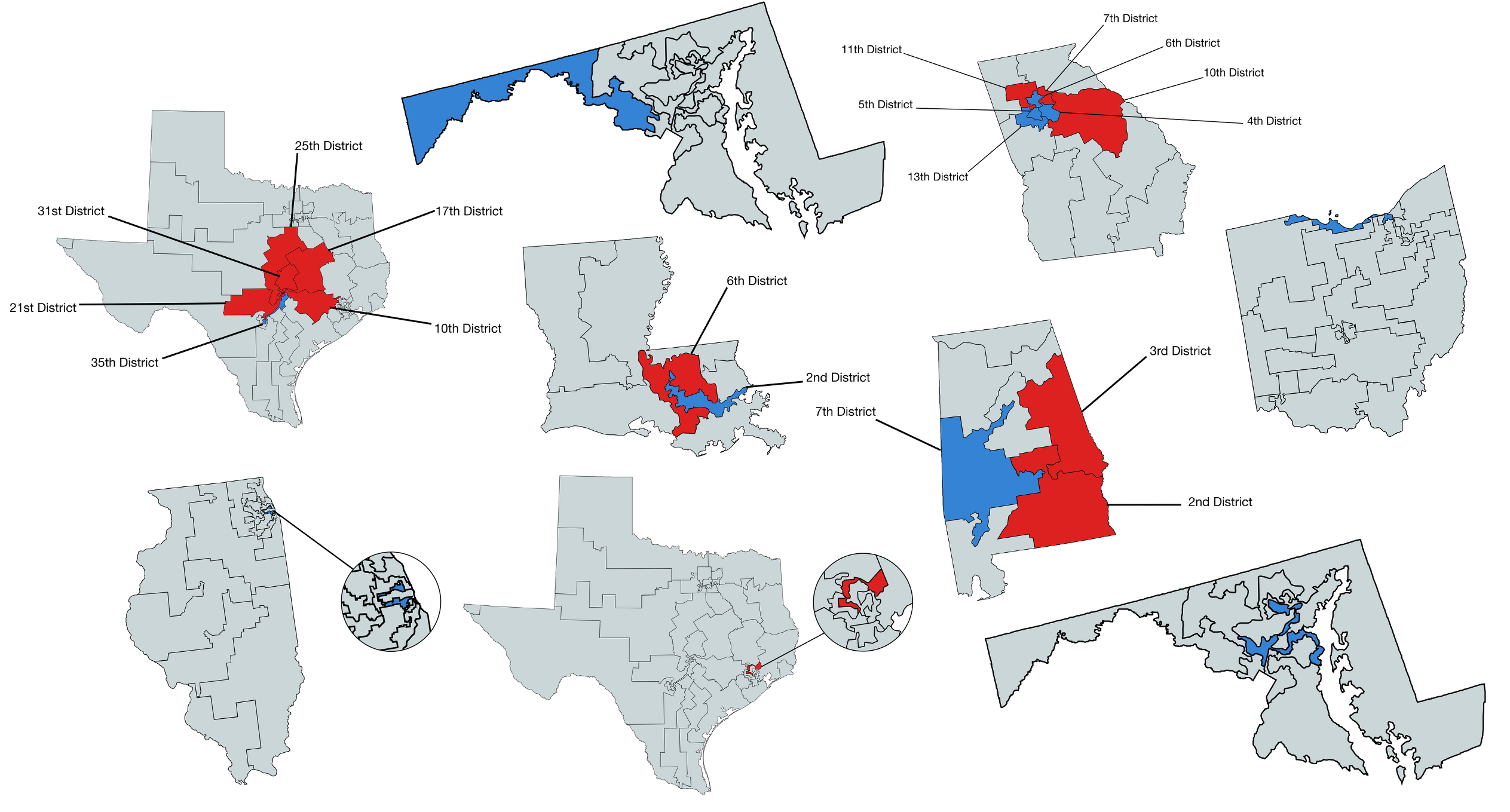
The MAUP occurs when the aggregate units of analysis are arbitrarily produced or not directly related to the underlying phenomena. A classic example of this problem is Gerrymandering.
Gerrymandering involves shaping and re-shaping voting districts based on the political affiliations of the resident citizenry.

Examples

Wrap up

Today we covered the following topics: - Spatial predicates and binary predicates - Spatial filtering and joining - Spatial simplification - Spatial tessellations / Coverages - Modifiable areal unit problem (MAUP)

Combined with your understanding of

Geometry and topology
Coordinate Reference Systems
Their integration with R

We are well suited to move on to raster data (gridded coverage model!) next week

Congrats!!

Last week

Measures (GEOS Measures)

For example …

Units

Topologic Diminsion

Predicates

Geometric Interiors, Boundaries and Exteriors

Interior, Boundary and Exterior: POINTS

Interior, Boundary and Exterior: LINESTRING

Interior, Boundary and Exterior: POLYGON

Summary

Predicates

Overlap is a POINT: 0D

Overlap is a LINESTRING: 1D

Overlap is a POLYGON: 2D

No Overlap = FALSE

Dimensionally Extended 9-Intersection Model

The Matrix Model

Illustration

Spatial Relations in R

Named Predicates

Binary Predicates

Named predicates in R

sparse matrix

dense matrix

st_relates vs. predicate calls…

So…

Filtering on data.frames

Spatial Filtering

Result

Distance Example (additional parameter)

Spatial Data Science

Spatial Joining

st_join

Every Starbucks in the World

Clipping

Spatial Subsetting

Simplification

Computational Complexity

Ramer–Douglas–Peucker

st_simplify

st_simplify

Visvalingam

rmapshaper

Tesselation

Core Concepts of Spatial Data: (Kuhn 2012)

Core Concepts of Spatial Data: (Kuhn 2012)

Core Concepts of Spatial Data: (Kuhn 2012)

Object View

Object View

Field View

Objects can provide coverage:

Object Coverages

LANDSAT Path Row

MODIS Sinisoial Grid

Uber Hex Addressing

what3word

Map Tiles / slippy maps / Pyramids

Our Data for today …

Southern Counties

Unioned to States using dplyr

South County Centroids

Southern Coverage: County

Regular Tiles

Southern Coverage: Square

Hexagonal Grid

Southern Coverage: Hexagon

Advantages Square Grids

Advantages Square Grids

Triangulations

Voronoi Polygons

Voronoi Polygons

Voronoi Polygons

Often used in numerical models and simulations

st_voronoi

Southern Coverage: Voronoi

Southern Coverage: Voronoi

Delaunay triangulation

Delaunay triangulation

Used in landscape evaluation and terrian modeling

Unioned to States using `dplyr`

`st_voronoi`

`st_triangulate`