Week 5

Machine Learning Part 1

Unit 3: Modeling (Machine Learning)

What is machine learning?

What is machine learning? (2025 edition)

Note

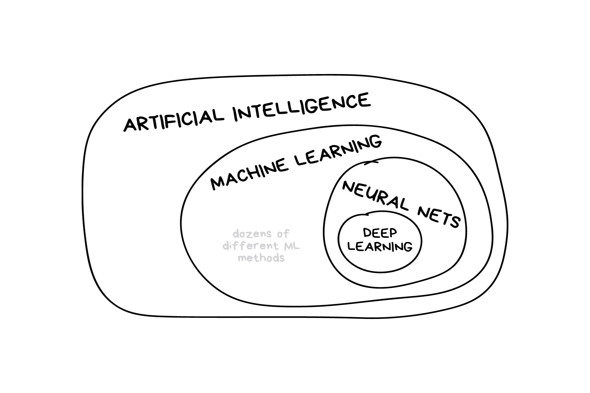
In the early 2010s, “Artificial intelligence” (AI) was largely synonymous with what we’ll refer to as “machine learning” in this workshop. In the late 2010s and early 2020s, AI usually referred to deep learning methods. Since the release of ChatGPT in late 2022, “AI” has come to also encompass large language models (LLMs) / generative models.

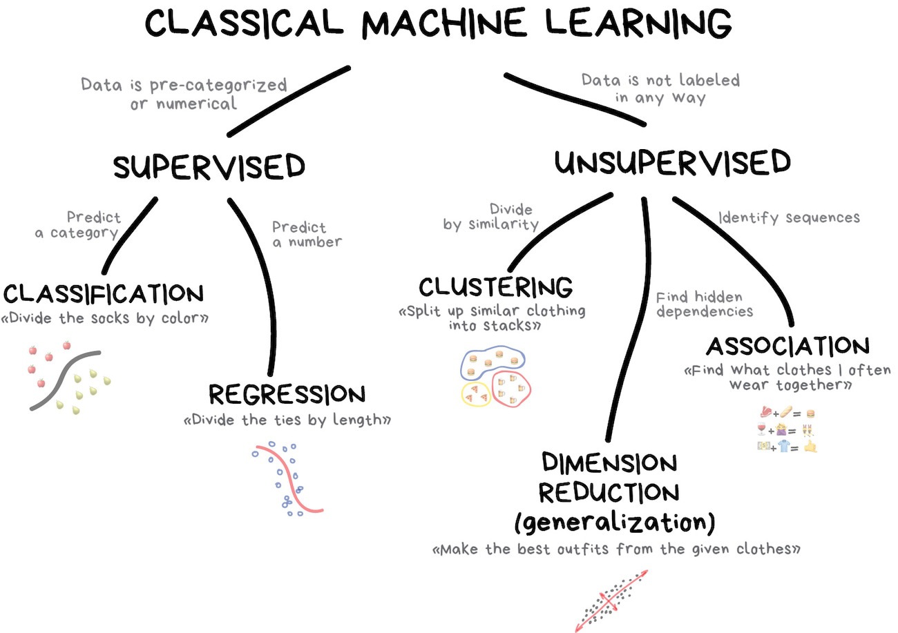
Classic Conceptual Model

The big picture: Road map

What is `tidymodels`?

An R package ecosystem for modeling and machine learning
Built on the tidyverse principles (consistent syntax, modular design)
Provides a structured workflow for preprocessing, model fitting, and evaluation
Includes packages for model specification, preprocessing, resampling, tuning, and evaluation
Promotes best practices for reproducibility and efficiency
Offers a unified interface for different models and tasks

Key tidymodels Packages

📦 recipes: Feature engineering and preprocessing

📦 parsnip: Unified interface for model specification

📦 workflows: Streamlined modeling pipelines

📦 tune: Hyperparameter tuning

📦 rsample: Resampling and validation

📦 yardstick: Model evaluation metrics

knitr::include_graphics('images/tidymodels-packages.png')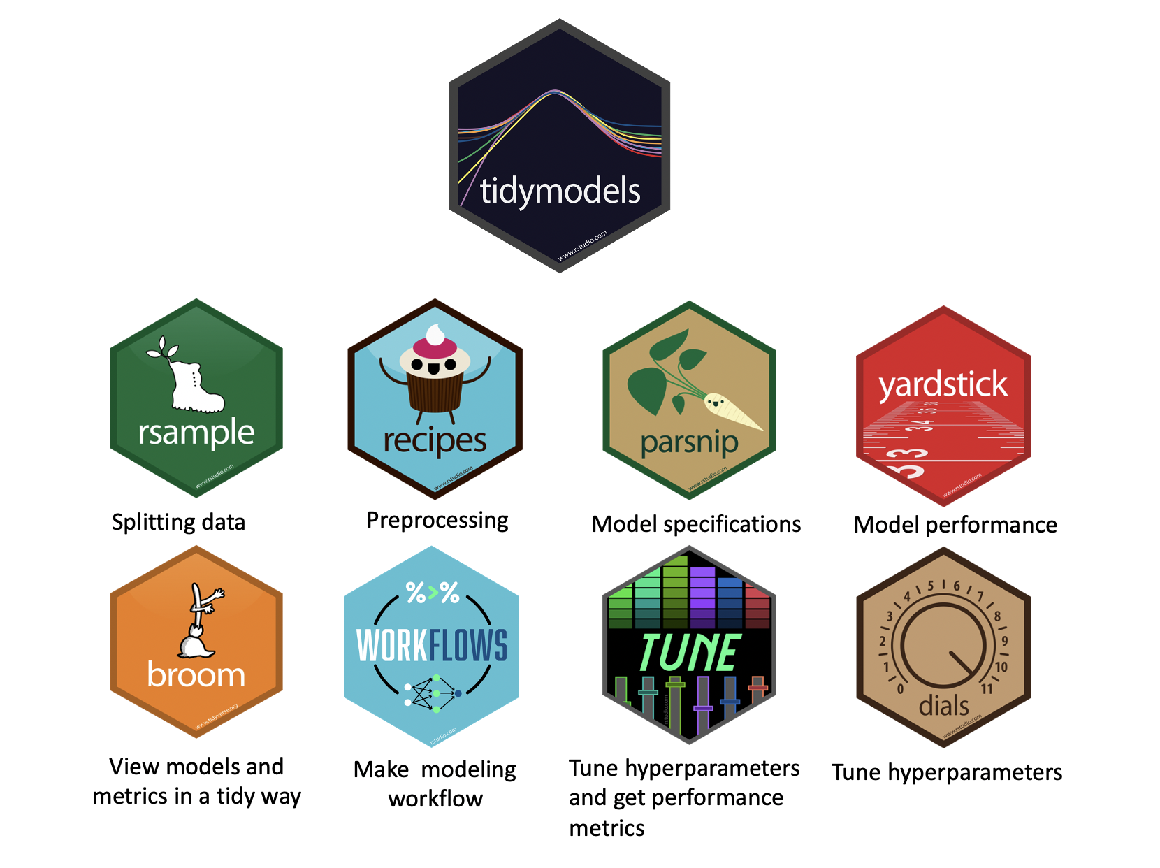

tidymodels::tidymodels_packages()
#>  [1] "broom"        "cli"          "conflicted"   "dials"        "dplyr"       
#>  [6] "ggplot2"      "hardhat"      "infer"        "modeldata"    "parsnip"     
#> [11] "purrr"        "recipes"      "rlang"        "rsample"      "rstudioapi"  
#> [16] "tibble"       "tidyr"        "tune"         "workflows"    "workflowsets"
#> [21] "yardstick"    "tidymodels"

Typcical Workflow in `tidymodels`

1️⃣ Load Package & Data

2️⃣ Preprocess Data (recipes)

3️⃣ Define Model (parsnip)

4️⃣ Create a Workflow (workflows)

5️⃣ Train & Tune (tune)

6️⃣ Evaluate Performance (yardstick)

Data Normalization: `tidymodels`

Data normalization is a crucial step in data preprocessing for machine learning.
It ensures that features contribute equally to model performance by transforming them into a common scale.
This is particularly important for algorithms that rely on distance metrics (e.g., k-nearest neighbors, support vector machines) or gradient-based optimization (e.g., neural networks, logistic regression).
In the tidymodels framework, data normalization is handled within preprocessing workflows using the recipes package, which provides a structured way to apply transformations consistently.

Why Normalize Data for ML?

✅ Improves Model Convergence: Many machine learning models rely on gradient descent, which can be inefficient if features are on different scales.

✅ Prevents Feature Domination: Features with large magnitudes can overshadow smaller ones, leading to biased models.

✅ Enhances Interpretability: Standardized data improves comparisons across variables and aids in better model understanding.

✅ Facilitates Distance-Based Methods: Algorithms like k-nearest neighbors and principal component analysis (PCA) perform best when data is normalized.

Common Normalization Techniques

1. `Min-Max Scaling`

Transforms data into a fixed range (typically [0,1]).
Preserves relationships but sensitive to outliers.
Formula: \[ x' = \frac{x - x_{min}}{x_{max} - x_{min}} \]
Implemented using step_range() in recipes.

2. `Z-Score Standardization (Standard Scaling)`

Centers data to have zero mean and unit variance.
More robust to outliers compared to min-max scaling.
Formula: \[ x' = \frac{x - \mu}{\sigma} \]
Implemented using step_normalize() in recipes.

Common Normalization Techniques

3. `Robust Scaling`

Uses median and interquartile range (IQR) for scaling.
Less sensitive to outliers.
Formula: \[ x' = \frac{x - median(x)}{IQR(x)} \]
Implemented using step_YeoJohnson() or step_BoxCox() in recipes.

4. `Log Transformation`

Useful for skewed distributions to reduce the impact of extreme values.
Implemented using step_log() in recipes.

Common Normalization Techniques

5. `Principal Component Analysis (PCA)`

Projects data into a lower-dimensional space while maintaining variance.
Used in high-dimensional datasets.
Implemented using step_pca() in recipes.

Other Feature Engineering Tasks

Handling Missing Data

step_impute_mean()
step_impute_median()
step_impute_knn()

can be used to fill missing values.

Encoding Categorical Variables

step_dummy() creates dummy variables for categorical features.
step_other() groups infrequent categories into an “other” category.

Creating Interaction Terms

step_interact() generates interaction terms between predictors.

Feature Extraction

step_pca() or step_ica() can be used to extract important components.

Text Feature Engineering

step_tokenize(), step_stopwords(), and step_tf() for text processing.

Binning Numerical Data

step_bin2factor() converts continuous variables into categorical bins.

Polynomial and Spline Features

step_poly() and step_bs() for generating polynomial and spline transformations.

Implementing Normalization in Tidymodels

What will we do?

We will create a recipe to normalize the numerical predictors in the penguins dataset using the recipes package.
We will then prepare (prep) the recipe and apply it to the dataset to obtain normalized data.
We will then bake the recipe to apply the transformations to the dataset.
Once processed, we can implement a linear regression model using the normalized data.

. . .

Example Workflow

library(tidymodels)

(recipe_obj <- recipe(flipper_length_mm ~ 
                       bill_length_mm + body_mass_g + 
                       sex + island + species, 
                      data = penguins) |> 
  step_impute_mean(all_numeric_predictors()) |>
  step_dummy(all_factor_predictors()) |>
  step_normalize(all_numeric_predictors()))

# Prepare and apply transformations
prep_recipe     <- prep(recipe_obj, training = penguins) 

normalized_data <- bake(prep_recipe, new_data = NULL) |> 
  mutate(species = penguins$species) |> 
  drop_na()

head(normalized_data)
#> # A tibble: 6 × 9
#>   bill_length_mm body_mass_g flipper_length_mm sex_male island_Dream
#>            <dbl>       <dbl>             <int>    <dbl>        <dbl>
#> 1         -0.886      -0.565               181    0.990       -0.750
#> 2         -0.812      -0.502               186   -1.01        -0.750
#> 3         -0.665      -1.19                195   -1.01        -0.750
#> 4         -1.33       -0.940               193   -1.01        -0.750
#> 5         -0.849      -0.690               190    0.990       -0.750
#> 6         -0.923      -0.721               181   -1.01        -0.750
#> # ℹ 4 more variables: island_Torgersen <dbl>, species_Chinstrap <dbl>,
#> #   species_Gentoo <dbl>, species <fct>

Explanation:

recipe() defines preprocessing steps for modeling.
step_impute_mean(all_numeric_predictors()) standardizes all numerical predictors.
step_dummy(all_factor_predictors()) creates dummy variables for categorical predictors.
step_normalize(all_numeric_predictors())) standardizes all numerical predictors.
prep() estimates parameters for transformations.
bake() applies the transformations to the dataset.

Build a model with Normalized Data

(model = lm(flipper_length_mm ~ . , data = normalized_data) )

#> 
#> Call:
#> lm(formula = flipper_length_mm ~ ., data = normalized_data)
#> 
#> Coefficients:
#>       (Intercept)     bill_length_mm        body_mass_g           sex_male  
#>          200.9649             2.2754             4.6414             0.7208  
#>      island_Dream   island_Torgersen  species_Chinstrap     species_Gentoo  
#>            0.6525             0.9800             0.5640             8.0796  
#>  speciesChinstrap      speciesGentoo  
#>                NA                 NA

Build a model with Normalized Data

(model = lm(flipper_length_mm ~ . , data = normalized_data) )

glance(model)

#> 
#> Call:
#> lm(formula = flipper_length_mm ~ ., data = normalized_data)
#> 
#> Coefficients:
#>       (Intercept)     bill_length_mm        body_mass_g           sex_male  
#>          200.9649             2.2754             4.6414             0.7208  
#>      island_Dream   island_Torgersen  species_Chinstrap     species_Gentoo  
#>            0.6525             0.9800             0.5640             8.0796  
#>  speciesChinstrap      speciesGentoo  
#>                NA                 NA
#> # A tibble: 1 × 12
#>   r.squared adj.r.squared sigma statistic   p.value    df logLik   AIC   BIC
#>       <dbl>         <dbl> <dbl>     <dbl>     <dbl> <dbl>  <dbl> <dbl> <dbl>
#> 1     0.863         0.861  5.23      294. 2.15e-136     7 -1020. 2057. 2092.
#> # ℹ 3 more variables: deviance <dbl>, df.residual <int>, nobs <int>

Build a model with Normalized Data

(model = lm(flipper_length_mm ~ . , data = normalized_data) )

glance(model)

(pred <- augment(model, normalized_data))

#> 
#> Call:
#> lm(formula = flipper_length_mm ~ ., data = normalized_data)
#> 
#> Coefficients:
#>       (Intercept)     bill_length_mm        body_mass_g           sex_male  
#>          200.9649             2.2754             4.6414             0.7208  
#>      island_Dream   island_Torgersen  species_Chinstrap     species_Gentoo  
#>            0.6525             0.9800             0.5640             8.0796  
#>  speciesChinstrap      speciesGentoo  
#>                NA                 NA
#> # A tibble: 1 × 12
#>   r.squared adj.r.squared sigma statistic   p.value    df logLik   AIC   BIC
#>       <dbl>         <dbl> <dbl>     <dbl>     <dbl> <dbl>  <dbl> <dbl> <dbl>
#> 1     0.863         0.861  5.23      294. 2.15e-136     7 -1020. 2057. 2092.
#> # ℹ 3 more variables: deviance <dbl>, df.residual <int>, nobs <int>
#> # A tibble: 333 × 15
#>    bill_length_mm body_mass_g flipper_length_mm sex_male island_Dream
#>             <dbl>       <dbl>             <int>    <dbl>        <dbl>
#>  1         -0.886      -0.565               181    0.990       -0.750
#>  2         -0.812      -0.502               186   -1.01        -0.750
#>  3         -0.665      -1.19                195   -1.01        -0.750
#>  4         -1.33       -0.940               193   -1.01        -0.750
#>  5         -0.849      -0.690               190    0.990       -0.750
#>  6         -0.923      -0.721               181   -1.01        -0.750
#>  7         -0.867       0.592               195    0.990       -0.750
#>  8         -0.518      -1.25                182   -1.01        -0.750
#>  9         -0.978      -0.502               191    0.990       -0.750
#> 10         -1.71        0.248               198    0.990       -0.750
#> # ℹ 323 more rows
#> # ℹ 10 more variables: island_Torgersen <dbl>, species_Chinstrap <dbl>,
#> #   species_Gentoo <dbl>, species <fct>, .fitted <dbl>, .resid <dbl>,
#> #   .hat <dbl>, .sigma <dbl>, .cooksd <dbl>, .std.resid <dbl>

Build a model with Normalized Data

(model = lm(flipper_length_mm ~ . , data = normalized_data) )

glance(model)

(pred <- augment(model, normalized_data))

ggscatter(pred,
          x = 'flipper_length_mm', y = '.fitted',
          add = "reg.line", conf.int = TRUE,
          cor.coef = TRUE, cor.method = "pearson",
          color = "species", palette = "jco")

#> 
#> Call:
#> lm(formula = flipper_length_mm ~ ., data = normalized_data)
#> 
#> Coefficients:
#>       (Intercept)     bill_length_mm        body_mass_g           sex_male  
#>          200.9649             2.2754             4.6414             0.7208  
#>      island_Dream   island_Torgersen  species_Chinstrap     species_Gentoo  
#>            0.6525             0.9800             0.5640             8.0796  
#>  speciesChinstrap      speciesGentoo  
#>                NA                 NA
#> # A tibble: 1 × 12
#>   r.squared adj.r.squared sigma statistic   p.value    df logLik   AIC   BIC
#>       <dbl>         <dbl> <dbl>     <dbl>     <dbl> <dbl>  <dbl> <dbl> <dbl>
#> 1     0.863         0.861  5.23      294. 2.15e-136     7 -1020. 2057. 2092.
#> # ℹ 3 more variables: deviance <dbl>, df.residual <int>, nobs <int>
#> # A tibble: 333 × 15
#>    bill_length_mm body_mass_g flipper_length_mm sex_male island_Dream
#>             <dbl>       <dbl>             <int>    <dbl>        <dbl>
#>  1         -0.886      -0.565               181    0.990       -0.750
#>  2         -0.812      -0.502               186   -1.01        -0.750
#>  3         -0.665      -1.19                195   -1.01        -0.750
#>  4         -1.33       -0.940               193   -1.01        -0.750
#>  5         -0.849      -0.690               190    0.990       -0.750
#>  6         -0.923      -0.721               181   -1.01        -0.750
#>  7         -0.867       0.592               195    0.990       -0.750
#>  8         -0.518      -1.25                182   -1.01        -0.750
#>  9         -0.978      -0.502               191    0.990       -0.750
#> 10         -1.71        0.248               198    0.990       -0.750
#> # ℹ 323 more rows
#> # ℹ 10 more variables: island_Torgersen <dbl>, species_Chinstrap <dbl>,
#> #   species_Gentoo <dbl>, species <fct>, .fitted <dbl>, .resid <dbl>,
#> #   .hat <dbl>, .sigma <dbl>, .cooksd <dbl>, .std.resid <dbl>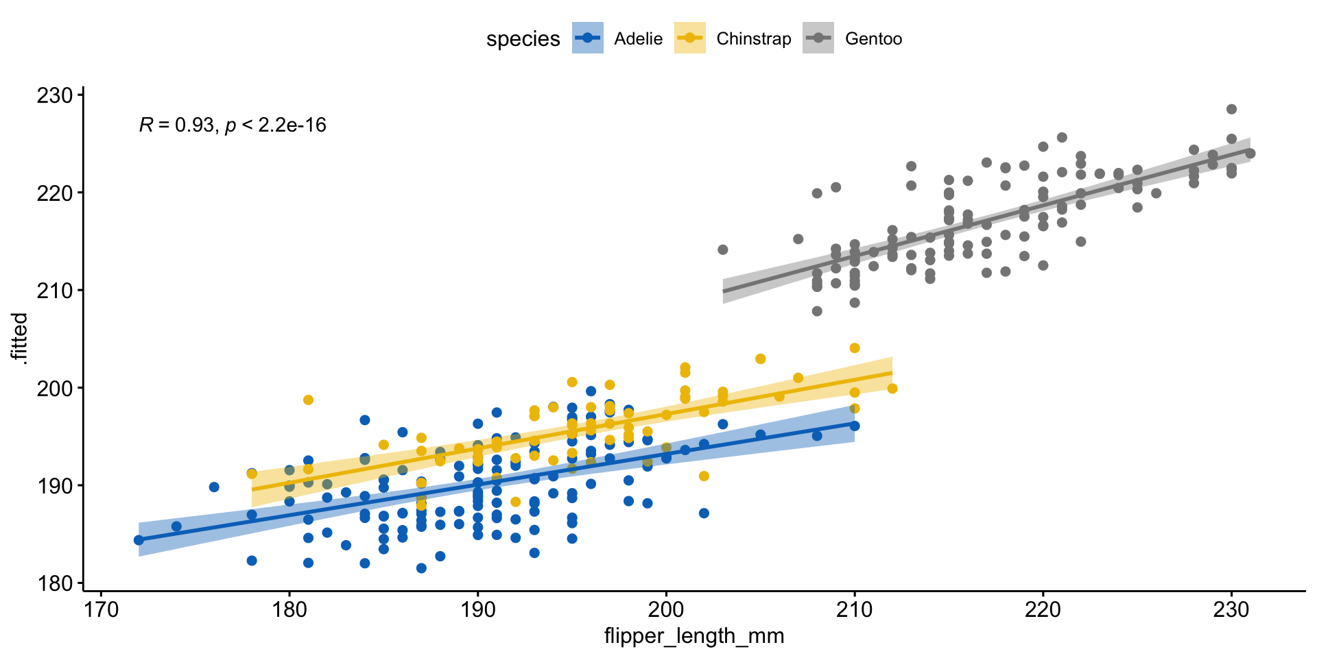

Data Budget

In any modeling effort, it’s crucial to evaluate the performance of a model using different validation techniques to ensure a model can generalize to unseen data.
But data is limited even in the age of “big data”.

Our typical process will like this:

Read in raw data (readr, dplyr::*_join) (single or multi table)

. . .

Prepare the data (EDA/mutate/summarize/clean, etc)

This is “Feature Engineering”

. . .

Once we’ve established our features (rows), we decide how to “spend” them …

. . .

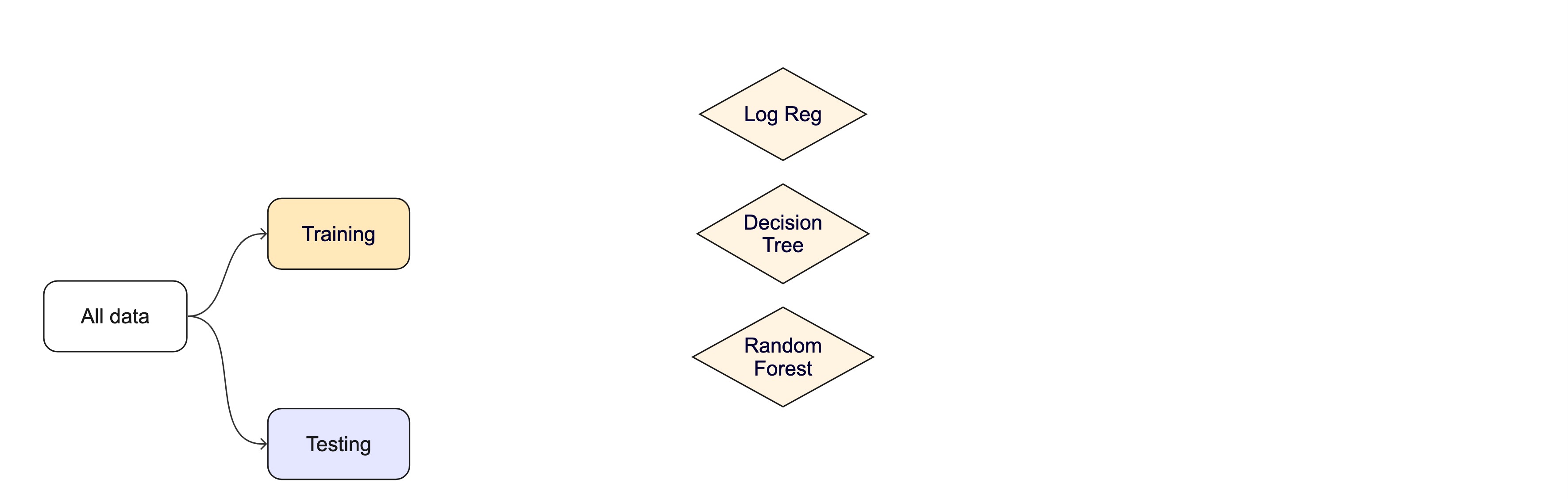
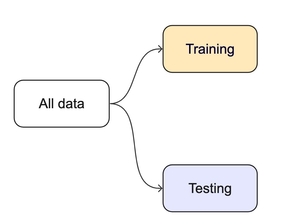
For machine learning, we typically split data into training and test sets:

. . .

The training set is used to estimate model parameters.
Spending too much data in training prevents us from computing a good assessment of model performance.

. . .

The test set is used as an independent assessment of performance.
Spending too much data in testing prevents us from computing good model parameter estimates.

How we split data

. . .

Splitting can be handled in many of ways. Typically, we base it off of a “hold out” percentage (e.g. 20%)
These hold out cases are extracted randomly from the data set. (remember seeds?)

. . .

The training set is usually the majority of the data and provides a sandbox for testing different modeling appraoches.

. . .

The test set is held in reserve until one or two models are chosen.
The test set is then used as the final arbiter to determine the efficacy of the model.

Startification

In many cases, there is a structure to the data that would inhibit inpartial spliiting (e.g. a class, a region, a species, a sex, etc)
Imagine you have a jar of M&Ms in different colors — red, blue, and green. You want to take some candies out to taste, but you want to make sure you get a fair mix of each color, not just grabbing a bunch of red ones by accident.
Stratified resampling is like making sure that if your jar is 50% red, 30% blue, and 20% green, then the handful of candies you take keeps the same balance.
In data science, we do the same thing when we pick samples from a dataset: we make sure that different groups (like categories of people, animals, or weather types) are still fairly represented!

Initial splits

In tidymodels, the rsample package provides functions for creating initial splits of data.
The initial_split() function is used to create a single split of the data.
The prop argument defines the proportion of the data to be used for training.
The default is 0.75, which means 75% of the data will be used for training and 25% for testing.

set.seed(101991)
(resample_split <- initial_split(penguins, prop = 0.8))
#> <Training/Testing/Total>
#> <275/69/344>

#Sanity check
69/344
#> [1] 0.2005814

Accessing the data:

Once the data is split, we can access the training and testing data using the training() and testing() functions to extract the partitioned data from the full set:

penguins_train <- training(resample_split)
glimpse(penguins_train)
#> Rows: 275
#> Columns: 7
#> $ species           <fct> Gentoo, Adelie, Gentoo, Chinstrap, Gentoo, Chinstrap…
#> $ island            <fct> Biscoe, Torgersen, Biscoe, Dream, Biscoe, Dream, Dre…
#> $ bill_length_mm    <dbl> 46.2, 43.1, 46.2, 45.9, 46.5, 48.1, 45.2, 55.9, 38.1…
#> $ bill_depth_mm     <dbl> 14.9, 19.2, 14.4, 17.1, 13.5, 16.4, 17.8, 17.0, 17.0…
#> $ flipper_length_mm <int> 221, 197, 214, 190, 210, 199, 198, 228, 181, 195, 20…
#> $ body_mass_g       <int> 5300, 3500, 4650, 3575, 4550, 3325, 3950, 5600, 3175…
#> $ sex               <fct> male, male, NA, female, female, female, female, male…

. . .

penguins_test <- testing(resample_split)
glimpse(penguins_test)
#> Rows: 69
#> Columns: 7
#> $ species           <fct> Adelie, Adelie, Adelie, Adelie, Adelie, Adelie, Adel…
#> $ island            <fct> Torgersen, Torgersen, Torgersen, Biscoe, Biscoe, Bis…
#> $ bill_length_mm    <dbl> NA, 39.3, 36.6, 35.9, 38.8, 37.9, 39.2, 39.6, 36.7, …
#> $ bill_depth_mm     <dbl> NA, 20.6, 17.8, 19.2, 17.2, 18.6, 21.1, 17.2, 18.8, …
#> $ flipper_length_mm <int> NA, 190, 185, 189, 180, 172, 196, 196, 187, 205, 187…
#> $ body_mass_g       <int> NA, 3650, 3700, 3800, 3800, 3150, 4150, 3550, 3800, …
#> $ sex               <fct> NA, male, female, female, male, female, male, female…

Proportional Gaps

# Dataset
(table(penguins$species) / nrow(penguins))
#> 
#>    Adelie Chinstrap    Gentoo 
#> 0.4418605 0.1976744 0.3604651
# Training Data
(table(penguins_train$species) / nrow(penguins_train))
#> 
#>    Adelie Chinstrap    Gentoo 
#> 0.4581818 0.1818182 0.3600000
# Testing Data
(table(penguins_test$species) / nrow(penguins_test))
#> 
#>    Adelie Chinstrap    Gentoo 
#> 0.3768116 0.2608696 0.3623188

Stratification Example

A stratified random sample conducts a specified split within defined subsets of subsets, and then pools the results.
Only one column can be used to define a strata but grouping/mutate opperations can be used to create a new column that can be used as a strata (e.g. species/island)
In the case of the penguins data, we can stratify by species (think back to our nested/linear model appraoch)
This ensures that the training and testing sets have the same proportion of each species as the original data.

# Set the seed
set.seed(123)

# Drop missing values and split the data
penguins <- drop_na(penguins)
penguins_strata <- initial_split(penguins, strata = species, prop = .8)

# Extract the training and testing sets

train_strata <- training(penguins_strata)
test_strata  <- testing(penguins_strata)

Proportional Alignment

# Check the proportions
# Dataset
table(penguins$species) / nrow(penguins)
#> 
#>    Adelie Chinstrap    Gentoo 
#> 0.4384384 0.2042042 0.3573574
# Training Data
table(train_strata$species) / nrow(train_strata)
#> 
#>    Adelie Chinstrap    Gentoo 
#> 0.4377358 0.2037736 0.3584906
# Testing Data
table(test_strata$species) / nrow(test_strata)
#> 
#>    Adelie Chinstrap    Gentoo 
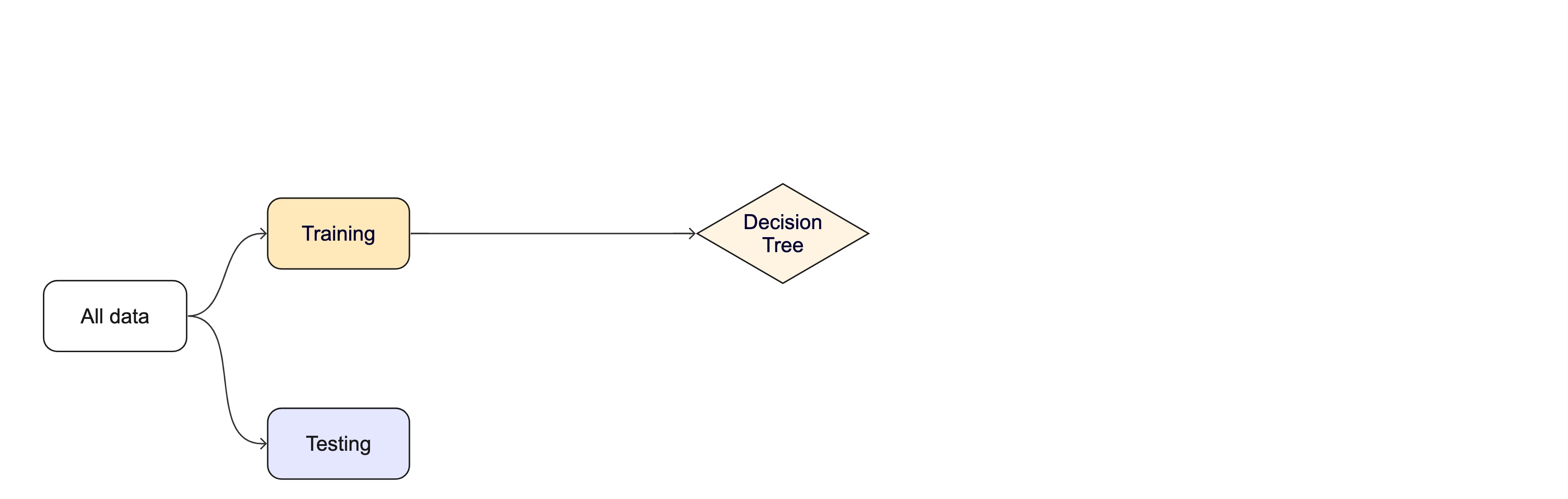
#> 0.4411765 0.2058824 0.3529412

Modeling

Once the data is split, we can decide what type of model to invoke.
Often, users simply pick a well known model type or class for a type of problem (Classic Conceptual Model)
We will learn more about model types and uses next week!
For now, just know that the training data is used to fit a model.
If we are certain about the model, we can use the test data to evaluate the model.

Modeling Options

But, there are many types of models, with different assumptions, behaviors, and qualities, that make some more applicable to a given dataset!
Most models have some type of parmeterization, that can often be tuned.
Testing combinations of model and tuning parmaters also requires some combintation of training/testing splits.

Modeling Options

What if we want to compare more models?

. . .

And/or more model configurations?

. . .

And we want to understand if these are important differences?

. . .

How can we use the training data to compare and evaluate different models? 🤔

. . .

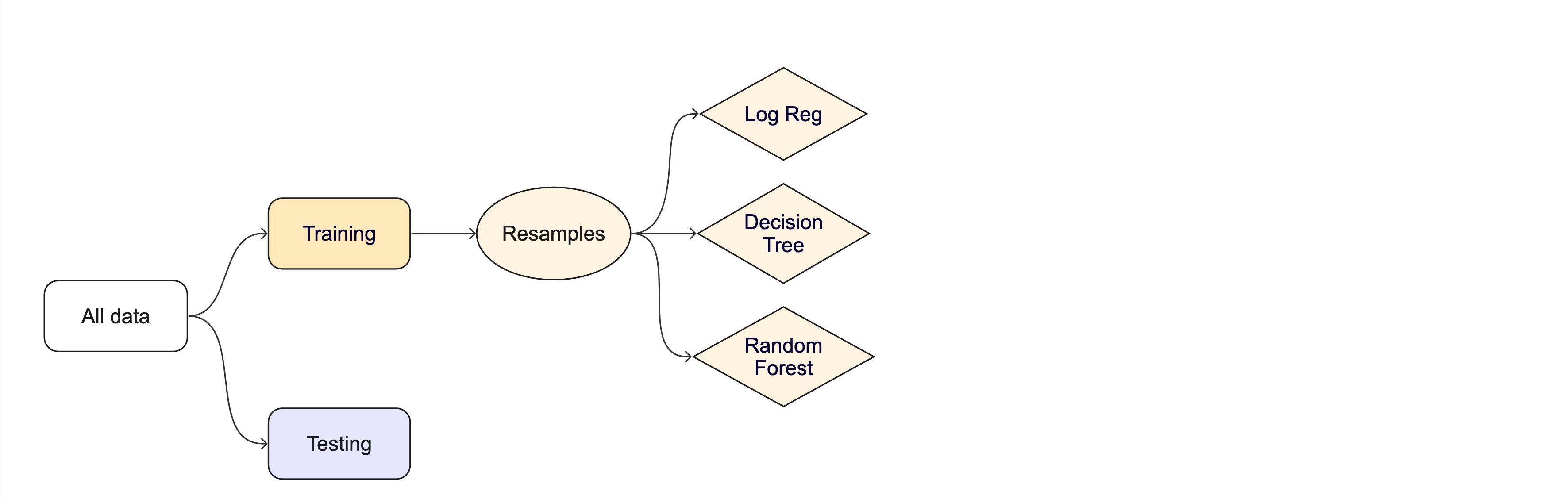
Resampling

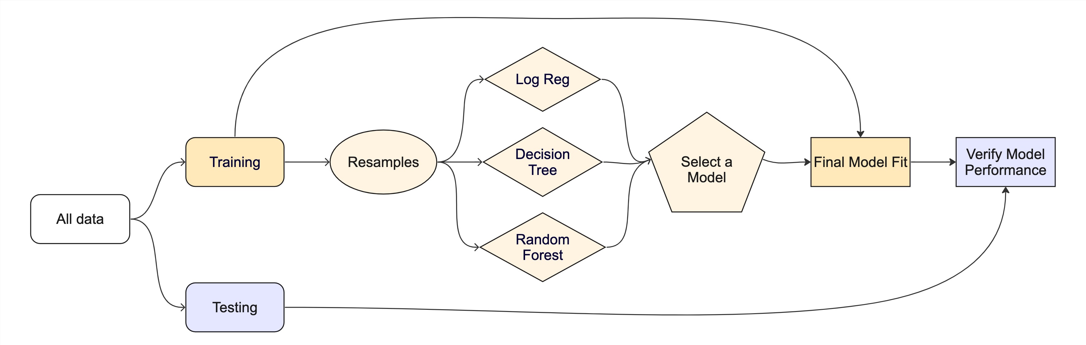
Testing combinations of model and tuning parmaters also requires some combintation of training/testing splits.
Resampling methods, such as cross-validation and bootstraping, are empirical simulation systems that help facilitate this.
They create a series of data sets similar to the initial training/testing split.
In the first level of the diagram to the right, we first split the original data into training/testing sets. Then, the training set is chosen for resampling.

Key Resampling Methods

Warning

Resampling is always used with the training set.

Resampling is a key step in model validation and assessment. The rsample package provides tools to create resampling strategies such as cross-validation, bootstrapping, and validation splits.

. . .

K-Fold Cross-Validation: The dataset is split into multiple “folds” (e.g., 5-fold or 10-fold), where each fold is used as a validation set while the remaining data is used for training.

. . .

Bootstrap Resampling: Samples are drawn with replacement from the training dataset to generate multiple datasets, which used to train and test the model.

. . .

Monte Carlo Resampling (Repeated Train-Test Splits): Randomly splits data multiple times.

. . .

Validation Split: Creates a single training and testing partition.

Cross-validation

penguins_train |> glimpse() 
#> Rows: 275
#> Columns: 7
#> $ species           <fct> Gentoo, Adelie, Gentoo, Chinstrap, Gentoo, Chinstrap…
#> $ island            <fct> Biscoe, Torgersen, Biscoe, Dream, Biscoe, Dream, Dre…
#> $ bill_length_mm    <dbl> 46.2, 43.1, 46.2, 45.9, 46.5, 48.1, 45.2, 55.9, 38.1…
#> $ bill_depth_mm     <dbl> 14.9, 19.2, 14.4, 17.1, 13.5, 16.4, 17.8, 17.0, 17.0…
#> $ flipper_length_mm <int> 221, 197, 214, 190, 210, 199, 198, 228, 181, 195, 20…
#> $ body_mass_g       <int> 5300, 3500, 4650, 3575, 4550, 3325, 3950, 5600, 3175…
#> $ sex               <fct> male, male, NA, female, female, female, female, male…

nrow(penguins_train) * 1/10
#> [1] 27.5

vfold_cv(penguins_train, v = 10) # v = 10 is default
#> #  10-fold cross-validation 
#> # A tibble: 10 × 2
#>    splits           id    
#>    <list>           <chr> 
#>  1 <split [247/28]> Fold01
#>  2 <split [247/28]> Fold02
#>  3 <split [247/28]> Fold03
#>  4 <split [247/28]> Fold04
#>  5 <split [247/28]> Fold05
#>  6 <split [248/27]> Fold06
#>  7 <split [248/27]> Fold07
#>  8 <split [248/27]> Fold08
#>  9 <split [248/27]> Fold09
#> 10 <split [248/27]> Fold10

Cross-validation

What is in this?

penguins_folds <- vfold_cv(penguins_train)
penguins_folds$splits[1:3]
#> [[1]]
#> <Analysis/Assess/Total>
#> <247/28/275>
#> 
#> [[2]]
#> <Analysis/Assess/Total>
#> <247/28/275>
#> 
#> [[3]]
#> <Analysis/Assess/Total>
#> <247/28/275>

Note

Here is another example of a list column enabling the storage of non-atomic types in tibble

Important

Set the seed when creating resamples

Alternate resampling schemes

Bootstrapping

set.seed(3214)
bootstraps(penguins_train)
#> # Bootstrap sampling 
#> # A tibble: 25 × 2
#>    splits            id         
#>    <list>            <chr>      
#>  1 <split [275/96]>  Bootstrap01
#>  2 <split [275/105]> Bootstrap02
#>  3 <split [275/108]> Bootstrap03
#>  4 <split [275/111]> Bootstrap04
#>  5 <split [275/102]> Bootstrap05
#>  6 <split [275/98]>  Bootstrap06
#>  7 <split [275/92]>  Bootstrap07
#>  8 <split [275/97]>  Bootstrap08
#>  9 <split [275/100]> Bootstrap09
#> 10 <split [275/99]>  Bootstrap10
#> # ℹ 15 more rows

Monte Carlo Cross-Validation

set.seed(322)
mc_cv(penguins_train, times = 10)
#> # Monte Carlo cross-validation (0.75/0.25) with 10 resamples  
#> # A tibble: 10 × 2
#>    splits           id        
#>    <list>           <chr>     
#>  1 <split [206/69]> Resample01
#>  2 <split [206/69]> Resample02
#>  3 <split [206/69]> Resample03
#>  4 <split [206/69]> Resample04
#>  5 <split [206/69]> Resample05
#>  6 <split [206/69]> Resample06
#>  7 <split [206/69]> Resample07
#>  8 <split [206/69]> Resample08
#>  9 <split [206/69]> Resample09
#> 10 <split [206/69]> Resample10

Validation set

set.seed(853)
penguins_val_split <- initial_validation_split(penguins)
penguins_val_split
#> <Training/Validation/Testing/Total>
#> <199/67/67/333>
validation_set(penguins_val_split)
#> # A tibble: 1 × 2
#>   splits           id        
#>   <list>           <chr>     
#> 1 <split [199/67]> validation

. . .

A validation set is just another type of resample

The whole game - status update

Unit Example

Can we predict if a plot of land is forested? - Interested in classification models - We have a dataset of 7,107 6000-acre hexagons in Washington state. - Each hexagon has a nominal outcome, forested, with levels "Yes" and "No".

Data on forests in Washington

The U.S. Forest Service maintains ML models to predict whether a plot of land is “forested.”
This classification is important for all sorts of research, legislation, and land management purposes.
Plots are typically remeasured every 10 years and this dataset contains the most recent measurement per plot.
Type ?forested to learn more about this dataset, including references.

Data on forests in Washington

library(tidymodels)
library(forested)
dim(forested)
#> [1] 7107   19

One observation from each of 7,107 6000-acre hexagons in Washington state.
A nominal outcome, forested, with levels "Yes" and "No", measured “on-the-ground.”

table(forested$forested)
#> 
#>  Yes   No 
#> 3894 3213

18 remotely-sensed and easily-accessible predictors:

names(forested)
#>  [1] "forested"         "year"             "elevation"        "eastness"        
#>  [5] "northness"        "roughness"        "tree_no_tree"     "dew_temp"        
#>  [9] "precip_annual"    "temp_annual_mean" "temp_annual_min"  "temp_annual_max" 
#> [13] "temp_january_min" "vapor_min"        "vapor_max"        "canopy_cover"    
#> [17] "lon"              "lat"              "land_type"

Data splitting and spending

The initial split

set.seed(123)
forested_split <- initial_split(forested, prop = .8, strata = tree_no_tree)
forested_split
#> <Training/Testing/Total>
#> <5685/1422/7107>

Accessing the data

forested_train <- training(forested_split)
forested_test  <- testing(forested_split)

nrow(forested_train)
#> [1] 5685
nrow(forested_test)
#> [1] 1422

K-Fold Cross-Validation

# Load the dataset
set.seed(123)

# Create a 10-fold cross-validation object
(forested_folds <- vfold_cv(forested_train, v = 10))
#> #  10-fold cross-validation 
#> # A tibble: 10 × 2
#>    splits             id    
#>    <list>             <chr> 
#>  1 <split [5116/569]> Fold01
#>  2 <split [5116/569]> Fold02
#>  3 <split [5116/569]> Fold03
#>  4 <split [5116/569]> Fold04
#>  5 <split [5116/569]> Fold05
#>  6 <split [5117/568]> Fold06
#>  7 <split [5117/568]> Fold07
#>  8 <split [5117/568]> Fold08
#>  9 <split [5117/568]> Fold09
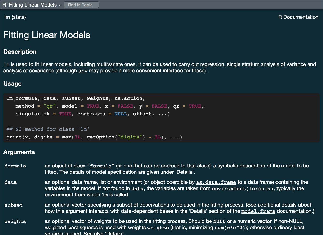
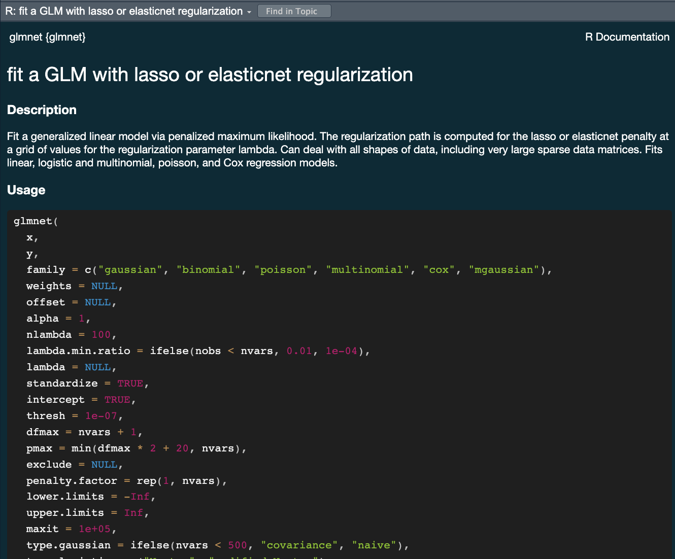
#> 10 <split [5117/568]> Fold10

How do you fit a linear model in R?

lm for linear model <– The one we have looked at!
glmnet for regularized regression
keras for regression using TensorFlow
stan for Bayesian regression using Stan
spark for large data sets using spark
brulee for regression using torch (PyTourch)

Challenge

All of these models have different syntax and functions
How do you keep track of all of them?
How do you know which one to use?
How would you compare them?

Comparing 3-5 of these models is a lot of work using functions for diverse packages.

The tidymodels advantage

In the tidymodels framework, all models are created using the same syntax:
- This makes it easy to compare models
- This makes it easy to switch between models
- This makes it easy to use the same model with different engines (packages)
The parsnip package provides a consistent interface to many models
For example, to fit a linear model you would be able to access the linear_reg() function

?linear_reg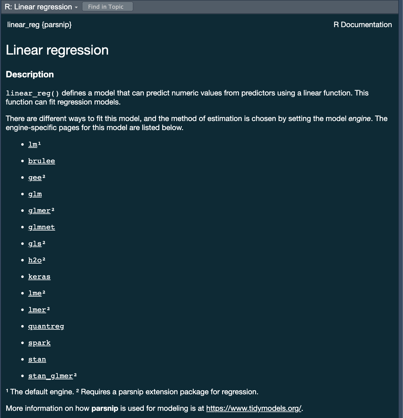

A tidymodels prediction will …

always be inside a tibble
have column names and types are unsurprising and predictable
ensure the number of rows in new_data and the output are the same

To specify a model

. . .

Choose a model
Specify an engine
Set the mode

Specify a model: Type

Next week we will discuss model types more thoroughly. For now, we will focus on two types:

Logistic Regression

logistic_reg()
#> Logistic Regression Model Specification (classification)
#> 
#> Computational engine: glm

decision_tree()
#> Decision Tree Model Specification (unknown mode)
#> 
#> Computational engine: rpart

We chose these two because they are robust, simple model that fit our goal of predicting a binary condition/class (forested/not forested)

Specify a model: engine

Choose a model
Specify an engine
Set the mode

?logistic_reg()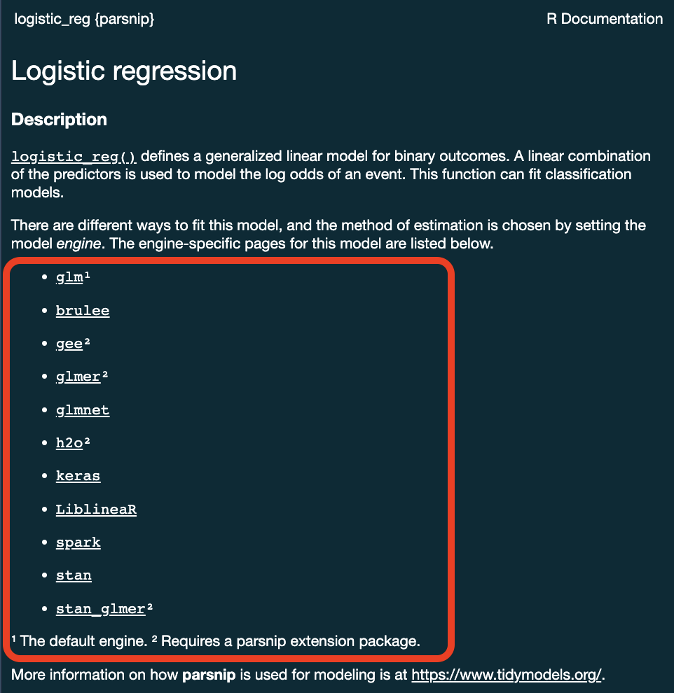

Specify a model: engine

logistic_reg() %>%
  set_engine("glmnet")
#> Logistic Regression Model Specification (classification)
#> 
#> Computational engine: glmnet

. . .

logistic_reg() %>%
  set_engine("stan")
#> Logistic Regression Model Specification (classification)
#> 
#> Computational engine: stan

Specify a model: mode

Choose a model
Specify an engine
Set the mode

?logistic_reg()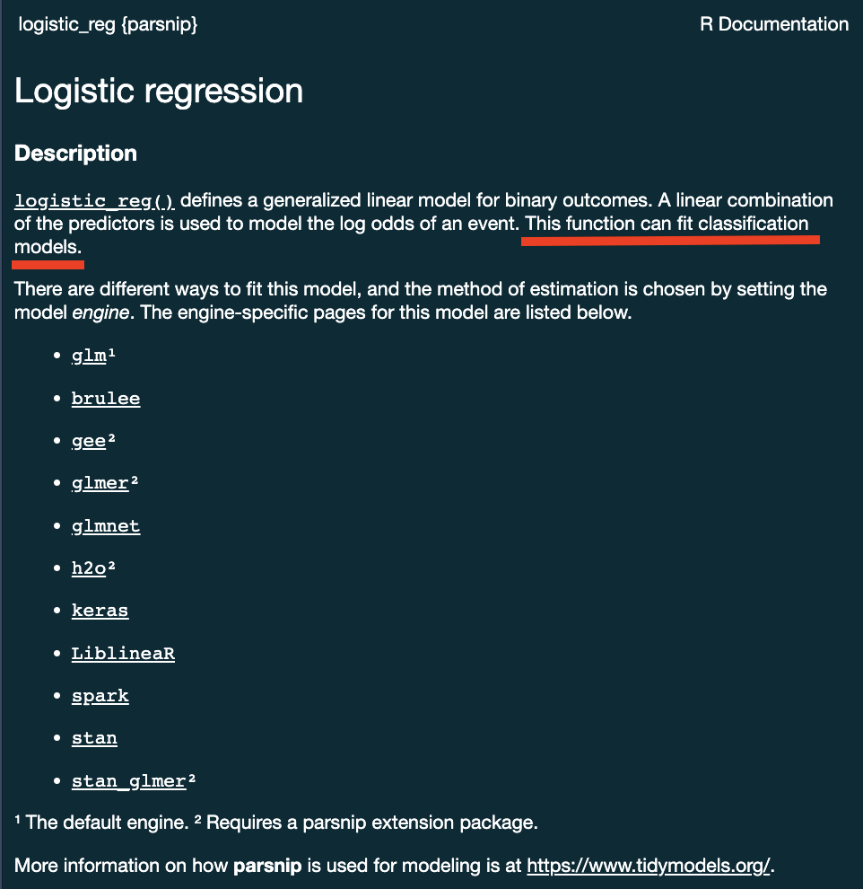

Specify a model: mode

Some models have limit classes …

logistic_reg() 
#> Logistic Regression Model Specification (classification)
#> 
#> Computational engine: glm

. . .

Others requires specification …

decision_tree()
#> Decision Tree Model Specification (unknown mode)
#> 
#> Computational engine: rpart

decision_tree() %>% 
  set_mode("classification")
#> Decision Tree Model Specification (classification)
#> 
#> Computational engine: rpart

All available models are listed at https://www.tidymodels.org/find/parsnip/

To specify a model

Choose a model
Specify an engine
Set the mode

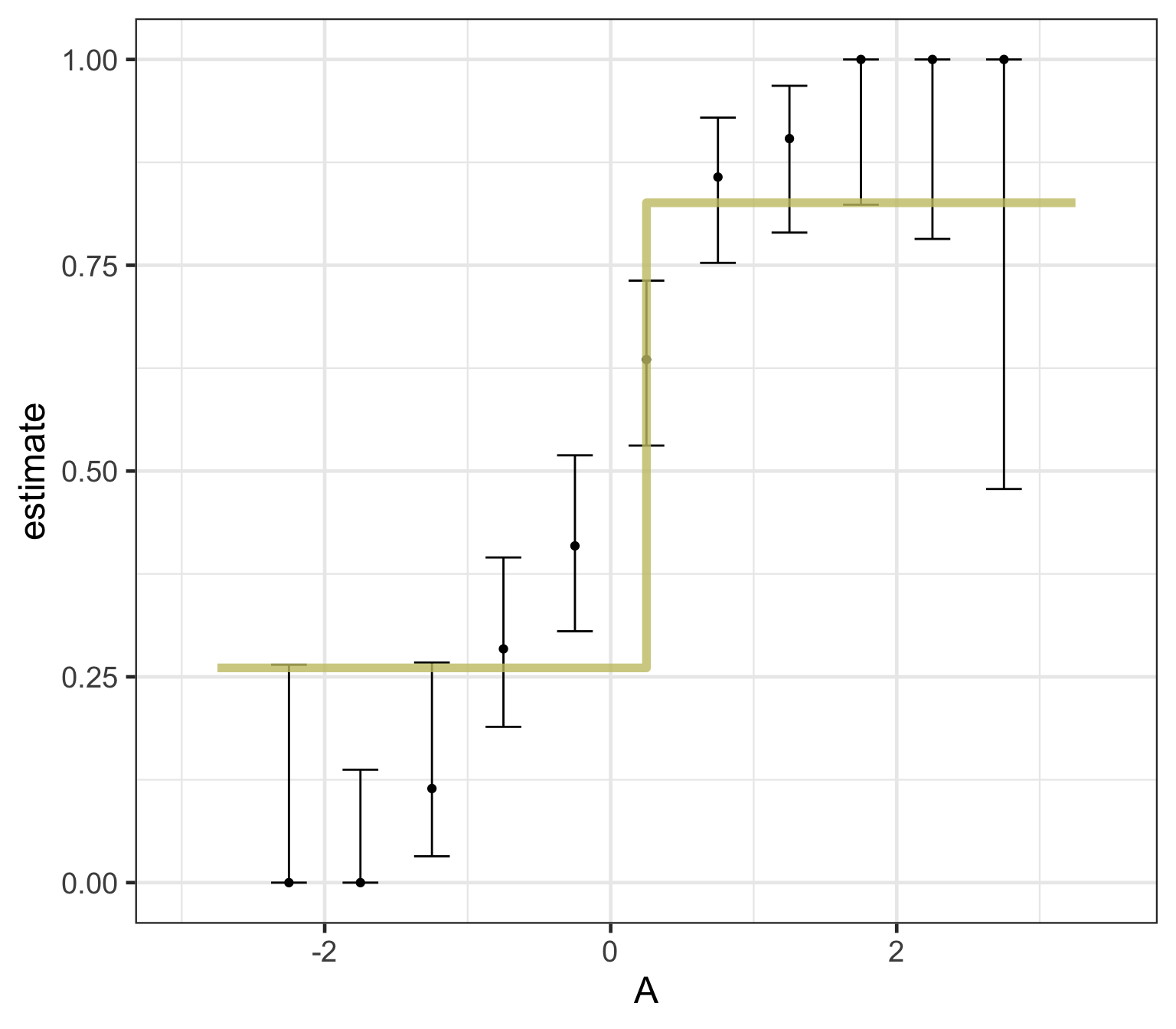
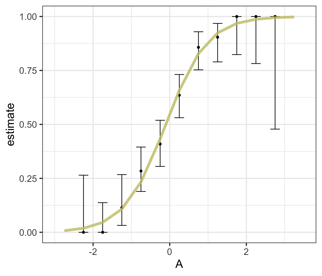
Logistic regression

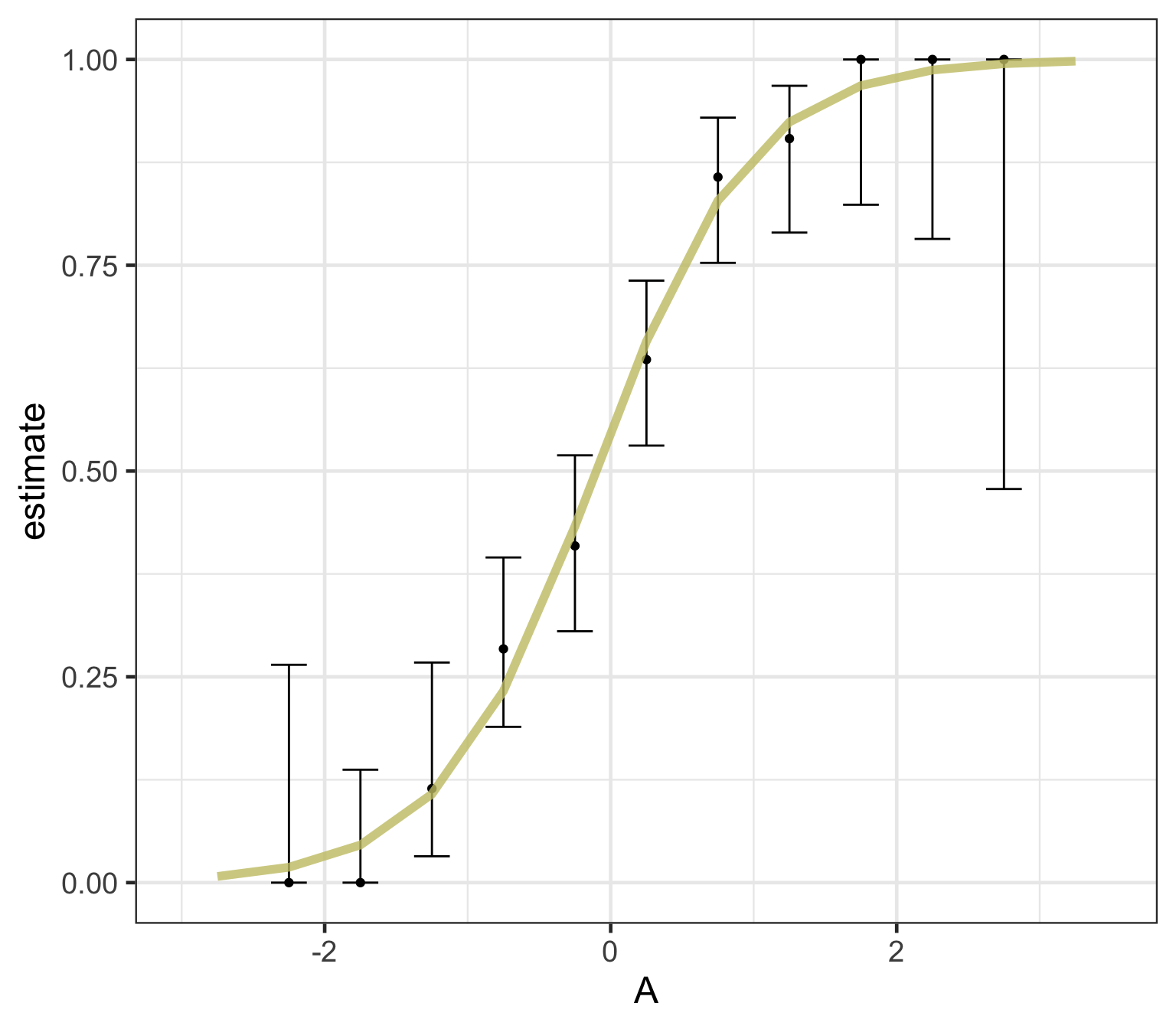
Logistic regression predicts probability—instead of a straight line, it gives an S-shaped curve that estimates how likely an outcome (e.g., is forested) is based on a predictor (e.g., rainfall and temperature).
The dots in the plot show the actual proportion of “successes” (e.g., is forested) within different bins of the predictor variable(s) (A).
The vertical error bars represent uncertainty—showing a range where the true probability might fall.
Logistic regression helps answer “how likely” questions—e.g., “How likely is someone to pass based on their study hours?” rather than just predicting a yes/no outcome.

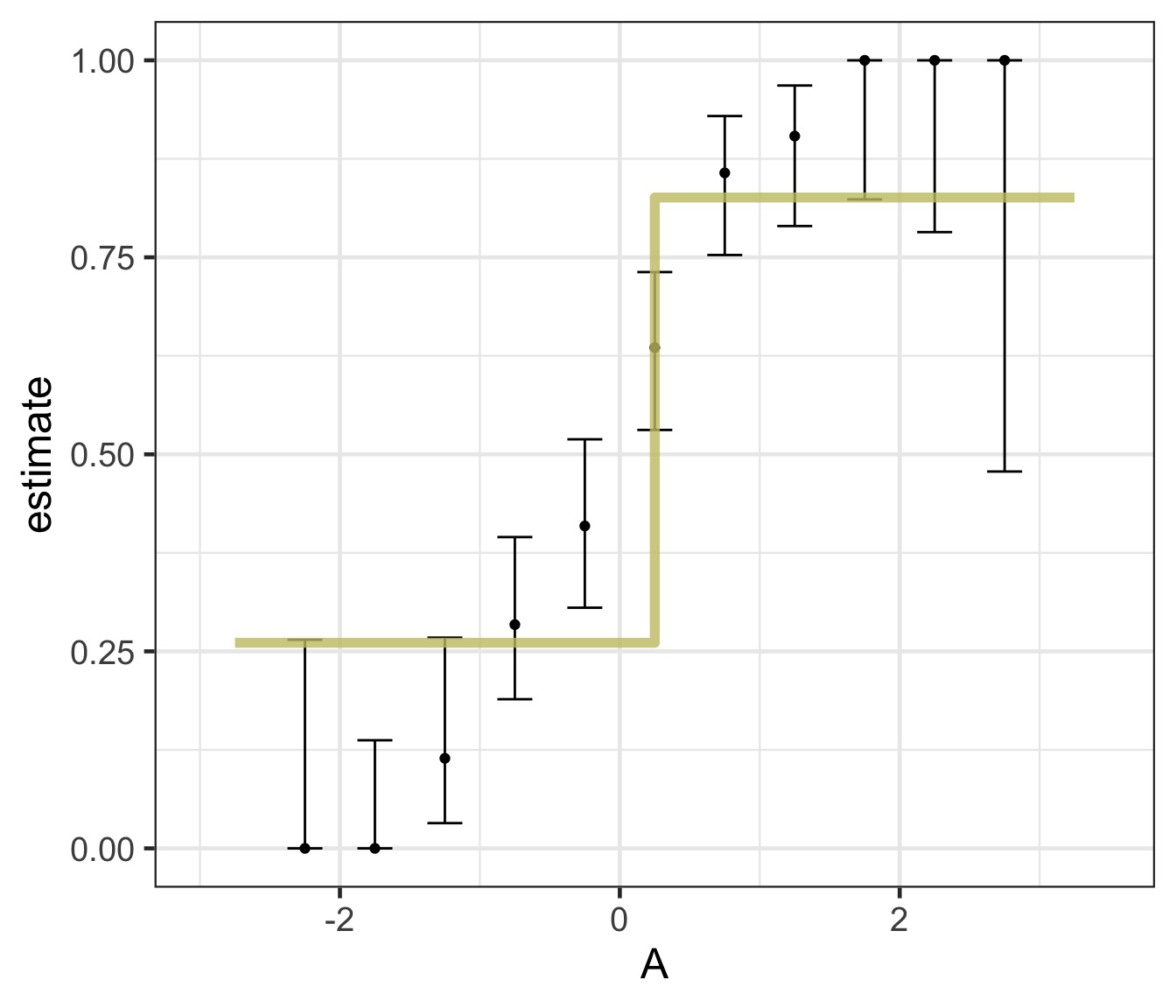
Decision trees

Decision trees

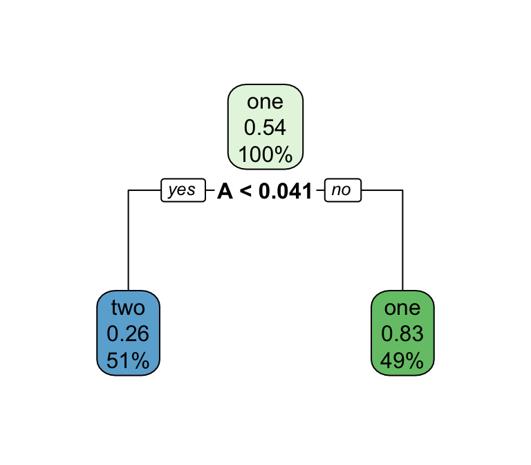
Series of splits or if/then statements based on predictors
First the tree grows until some condition is met (maximum depth, no more data)
Then the tree is pruned to reduce its complexity

Decision trees

What algorithm is best for estimate forested plots?

We can only really know by testing them …

Logistic regression

Decision trees

Fitting your model:

OK! So you have split data, you have a model, and you have an engine and mode
Now you need to fit the model!
This is done using the fit() function

dt_model <- decision_tree() %>% 
  set_engine('rpart') %>%
  set_mode("classification")

# Model, formula, data inputs
(output <- fit(dt_model, forested ~ ., data = forested_train) )
#> parsnip model object
#> 
#> n= 5685 
#> 
#> node), split, n, loss, yval, (yprob)
#>       * denotes terminal node
#> 
#>  1) root 5685 2571 Yes (0.54775726 0.45224274)  
#>    2) land_type=Tree 3025  289 Yes (0.90446281 0.09553719) *
#>    3) land_type=Barren,Non-tree vegetation 2660  378 No (0.14210526 0.85789474)  
#>      6) temp_annual_max< 13.395 351  155 Yes (0.55840456 0.44159544)  
#>       12) tree_no_tree=Tree 91    5 Yes (0.94505495 0.05494505) *
#>       13) tree_no_tree=No tree 260  110 No (0.42307692 0.57692308) *
#>      7) temp_annual_max>=13.395 2309  182 No (0.07882200 0.92117800) *

Component extracts:

While tidymodels provides a standard interface to all models all base models have specific methods (remember summary.lm? )
To use these, you must extract a the underlying object.
extract_fit_engine() extracts the underlying model object
extract_fit_parsnip() extracts the parsnip object
extract_recipe() extracts the recipe object
extract_preprocessor() extracts the preprocessor object
… many more

ex <- extract_fit_engine(output)
class(ex) # the class of the engine used!
#> [1] "rpart"

# Use rpart plot and text methods ...
plot(ex)
text(ex, cex = 0.9, use.n = TRUE, xpd = TRUE,)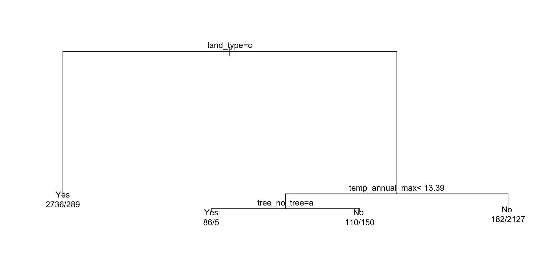

A model workflow

Workflows?

The workflows package in tidymodels helps:

Manage preprocessing and modeling in a structured pipeline
Avoid repetitive code
Reduce errors when integrating steps

. . .

Think of them as containers for:

Preprocessing steps (e.g., feature engineering, transformations)
Model specification
Fitting approaches

. . .

Why Use Workflows?

✅ Keeps preprocessing and modeling together

✅ Ensures consistency in data handling

✅ Makes code easier to read and maintain

Basic Workflow Structure:

Create a workflow object (similar to how ggplot() instantiates a canvas)
Add a formula or recipe (preprocessor)
Add the model
Fit the workflow

A model workflow

dt_wf <- workflow() %>%
  add_formula(forested ~ .) %>%
  add_model(dt_model) %>%
  fit(data = forested_train)

#> ══ Workflow [trained] ══════════════════════════════════════════════════════════
#> Preprocessor: Formula
#> Model: decision_tree()
#> 
#> ── Preprocessor ────────────────────────────────────────────────────────────────
#> forested ~ .
#> 
#> ── Model ───────────────────────────────────────────────────────────────────────
#> n= 5685 
#> 
#> node), split, n, loss, yval, (yprob)
#>       * denotes terminal node
#> 
#>  1) root 5685 2571 Yes (0.54775726 0.45224274)  
#>    2) land_type=Tree 3025  289 Yes (0.90446281 0.09553719) *
#>    3) land_type=Barren,Non-tree vegetation 2660  378 No (0.14210526 0.85789474)  
#>      6) temp_annual_max< 13.395 351  155 Yes (0.55840456 0.44159544)  
#>       12) tree_no_tree=Tree 91    5 Yes (0.94505495 0.05494505) *
#>       13) tree_no_tree=No tree 260  110 No (0.42307692 0.57692308) *
#>      7) temp_annual_max>=13.395 2309  182 No (0.07882200 0.92117800) *

Predict with your model

How do you use your new model?

augment() will return the dataset with predictions and residuals added.

dt_preds <- augment(dt_wf, new_data = forested_test)

#> # A tibble: 1,422 × 22
#>    .pred_class .pred_Yes .pred_No forested  year elevation eastness northness
#>    <fct>           <dbl>    <dbl> <fct>    <dbl>     <dbl>    <dbl>     <dbl>
#>  1 Yes            0.904    0.0955 No        2005       164      -84        53
#>  2 Yes            0.904    0.0955 Yes       2005       806       47       -88
#>  3 No             0.423    0.577  Yes       2005      2240      -67       -74
#>  4 Yes            0.904    0.0955 Yes       2005       787       66       -74
#>  5 Yes            0.904    0.0955 Yes       2005      1330       99         7
#>  6 Yes            0.904    0.0955 Yes       2005      1423       46        88
#>  7 Yes            0.904    0.0955 Yes       2014       546      -92       -38
#>  8 Yes            0.904    0.0955 Yes       2014      1612       30       -95
#>  9 No             0.0788   0.921  No        2014       235        0      -100
#> 10 No             0.0788   0.921  No        2014       308      -70       -70
#> # ℹ 1,412 more rows
#> # ℹ 14 more variables: roughness <dbl>, tree_no_tree <fct>, dew_temp <dbl>,
#> #   precip_annual <dbl>, temp_annual_mean <dbl>, temp_annual_min <dbl>,
#> #   temp_annual_max <dbl>, temp_january_min <dbl>, vapor_min <dbl>,
#> #   vapor_max <dbl>, canopy_cover <dbl>, lon <dbl>, lat <dbl>, land_type <fct>

Evaluate your model

How do you evaluate the skill of your models?

We will learn more about model evaluation and tuning latter in this unit, but for now we can blindly use the metrics() function defaults to get a sense of how our model is doing.

The default metrics for classification models are accuracy and kap (Cohen’s Kappa)
The default metric for regression models are RMSE, R^2, and MAE

# We have a classification model
metrics(dt_preds, truth = forested, estimate = .pred_class)
#> # A tibble: 2 × 3
#>   .metric  .estimator .estimate
#>   <chr>    <chr>          <dbl>
#> 1 accuracy binary         0.885
#> 2 kap      binary         0.768

`tidymodels` advantage!

OK! while that was not too much work, it certainly wasn’t minimal.

. . .

Now lets say you want to check if the logistic regression model performs better than the decision tree
That sounds like a lot to repeat.
Fortunately, the tidymodels framework makes this a straight forward swap!

. . .

log_mod = logistic_reg() %>% 
  set_engine("glm") %>% 
  set_mode("classification")

log_wf <- workflow() %>%
  add_formula(forested ~ .) %>%
  add_model(log_mod) %>%
  fit(data = forested_train)

log_preds <- augment(log_wf, new_data = forested_test)

metrics(log_preds, truth = forested, estimate = .pred_class)
#> # A tibble: 2 × 3
#>   .metric  .estimator .estimate
#>   <chr>    <chr>          <dbl>
#> 1 accuracy binary         0.890
#> 2 kap      binary         0.777

So who wins?

metrics(dt_preds, truth = forested, estimate = .pred_class)
#> # A tibble: 2 × 3
#>   .metric  .estimator .estimate
#>   <chr>    <chr>          <dbl>
#> 1 accuracy binary         0.885
#> 2 kap      binary         0.768
metrics(log_preds, truth = forested, estimate = .pred_class)
#> # A tibble: 2 × 3
#>   .metric  .estimator .estimate
#>   <chr>    <chr>          <dbl>
#> 1 accuracy binary         0.890
#> 2 kap      binary         0.777

Right out of the gate, there doesn’t seem to be much difference, but …

Don’t get to confident!

We have evaluated the model on the same data we trained it on
This is not a good practice and can give us a false sense of confidence
Instead, we can use our resamples to better understand the skill of a model based on the iterative leave out policy:

dt_wf_rs <- workflow() %>%
  add_formula(forested ~ .) %>%
  add_model(dt_model) %>%
  fit_resamples(resamples = forested_folds, 
                # Here we just ask tidymodels to save all predictions...
                control   = control_resamples(save_pred = TRUE))

#> # A tibble: 1 × 5
#>   splits             id     .metrics         .notes           .predictions      
#>   <list>             <chr>  <list>           <list>           <list>            
#> 1 <split [5116/569]> Fold01 <tibble [3 × 4]> <tibble [0 × 3]> <tibble [569 × 6]>

Note

tidyr::unnest could be used to expand any of those list columns!

Don’t get to confident!

We can execute the same workflow for the logistic regression model, this time evaluating the resamples instead of the test data.

log_wf_rs <- workflow() %>%
  add_formula(forested ~ .) %>%
  add_model(log_mod) %>%
  fit_resamples(resamples = forested_folds,
                control = control_resamples(save_pred = TRUE))

#> # Resampling results
#> # 10-fold cross-validation 
#> # A tibble: 10 × 5
#>    splits             id     .metrics         .notes           .predictions
#>    <list>             <chr>  <list>           <list>           <list>      
#>  1 <split [5116/569]> Fold01 <tibble [3 × 4]> <tibble [0 × 3]> <tibble>    
#>  2 <split [5116/569]> Fold02 <tibble [3 × 4]> <tibble [0 × 3]> <tibble>    
#>  3 <split [5116/569]> Fold03 <tibble [3 × 4]> <tibble [0 × 3]> <tibble>    
#>  4 <split [5116/569]> Fold04 <tibble [3 × 4]> <tibble [0 × 3]> <tibble>    
#>  5 <split [5116/569]> Fold05 <tibble [3 × 4]> <tibble [0 × 3]> <tibble>    
#>  6 <split [5117/568]> Fold06 <tibble [3 × 4]> <tibble [0 × 3]> <tibble>    
#>  7 <split [5117/568]> Fold07 <tibble [3 × 4]> <tibble [0 × 3]> <tibble>    
#>  8 <split [5117/568]> Fold08 <tibble [3 × 4]> <tibble [0 × 3]> <tibble>    
#>  9 <split [5117/568]> Fold09 <tibble [3 × 4]> <tibble [0 × 3]> <tibble>    
#> 10 <split [5117/568]> Fold10 <tibble [3 × 4]> <tibble [0 × 3]> <tibble>

Don’t get to confident!

Since we now have an “ensemble” of models (across the folds), we can collect a summary of the metrics across them.
The default metrics for classification ensembles are:
- accuracy: accuracy is the proportion of correct predictions
- brier_class: the Brier score for classification is the mean squared difference between the predicted probability and the actual outcome
- roc_auc: the area under the ROC (Receiver Operating Characteristic) curve


collect_metrics(log_wf_rs)
#> # A tibble: 3 × 6
#>   .metric     .estimator   mean     n std_err .config             
#>   <chr>       <chr>       <dbl> <int>   <dbl> <chr>               
#> 1 accuracy    binary     0.906     10 0.00360 Preprocessor1_Model1
#> 2 brier_class binary     0.0714    10 0.00191 Preprocessor1_Model1
#> 3 roc_auc     binary     0.961     10 0.00164 Preprocessor1_Model1
collect_metrics(dt_wf_rs)
#> # A tibble: 3 × 6
#>   .metric     .estimator   mean     n std_err .config             
#>   <chr>       <chr>       <dbl> <int>   <dbl> <chr>               
#> 1 accuracy    binary     0.896     10 0.00385 Preprocessor1_Model1
#> 2 brier_class binary     0.0889    10 0.00224 Preprocessor1_Model1
#> 3 roc_auc     binary     0.909     10 0.00267 Preprocessor1_Model1

Further simplification: `workflowsets`

OK, so we have streamlined a lot of things with tidymodels:

We have a specified preprocesser (e.g. formula or recipe)
We have defined a model (complete with engine and mode)
We have implemented workflows pairing each model with the preprocesser to either fit the model to the resamples, or, the training data.

While a significant improvement, we can do better!

Does the idea of implementing a process over an list of elements ring a bell?

Model mappings:

workflowsets is a package that builds off of purrr and allows you to iterate over multiple models and/or multiple resamples
Remember how map, map_*, map2, and walk2 functions allow lists to map to lists or vectors? workflow_set maps a preprocessor (formula or recipe) to a set of models - each provided as a list object.
To start, we will create a workflow_set object (instead of a workflow). The first argument is a list of preprocessor objects (formulas or recipes) and the second argument is a list of model objects.
Both must be lists, by nature of the underlying purrr code.

(wf_obj <- workflow_set(list(forested ~.), list(log_mod, dt_model)))
#> # A workflow set/tibble: 2 × 4
#>   wflow_id              info             option    result    
#>   <chr>                 <list>           <list>    <list>    
#> 1 formula_logistic_reg  <tibble [1 × 4]> <opts[0]> <list [0]>
#> 2 formula_decision_tree <tibble [1 × 4]> <opts[0]> <list [0]>

Iteritive extecution

Once the workflow_set object is created, the workflow_map function can be used to map a function across the preprocessor/model combinations.
Here we are mapping the fit_resamples function across the workflow_set combinations using the resamples argument to specify the resamples we want to use (forested_folds).

wf_obj <- 
  workflow_set(list(forested ~.), list(log_mod, dt_model)) %>%
  workflow_map("fit_resamples", resamples = forested_folds)

#> # A workflow set/tibble: 2 × 4
#>   wflow_id              info             option    result   
#>   <chr>                 <list>           <list>    <list>   
#> 1 formula_logistic_reg  <tibble [1 × 4]> <opts[1]> <rsmp[+]>
#> 2 formula_decision_tree <tibble [1 × 4]> <opts[1]> <rsmp[+]>

Rapid comparision

With that single function, all models have been fit to the resamples and we can quickly compare the results both graphically and statistically:

# Quick plot function
autoplot(wf_obj) + 
  theme_linedraw()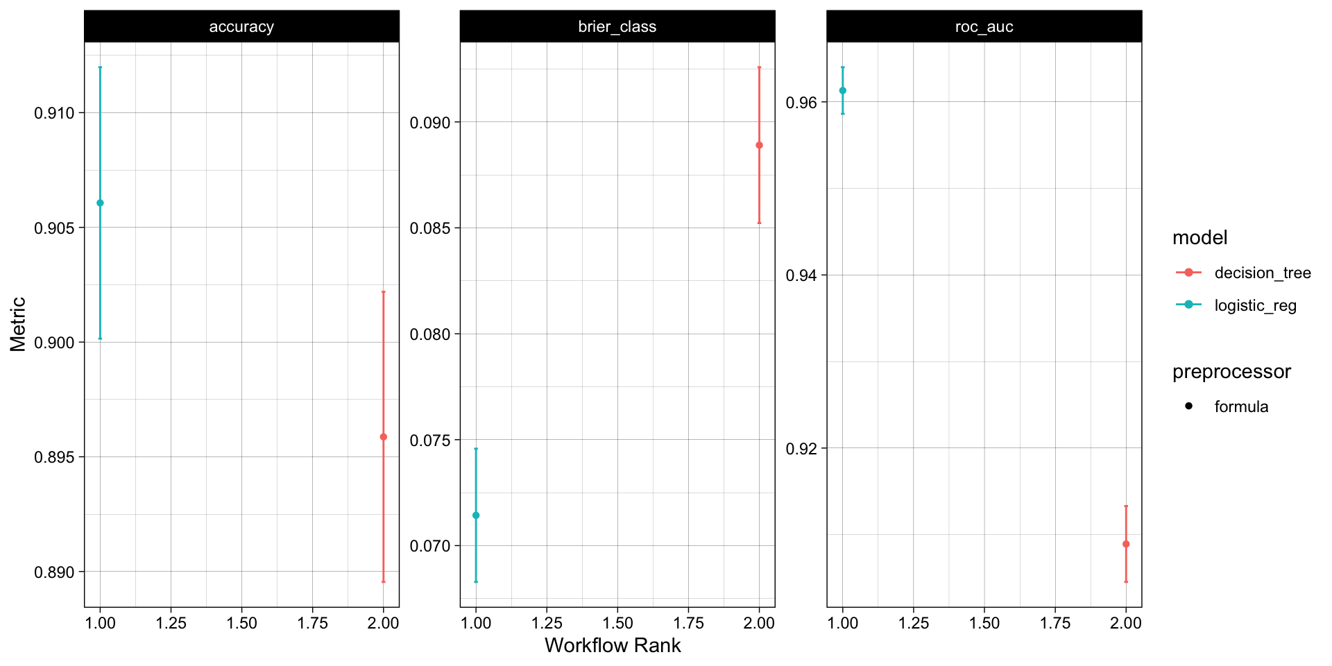

# Long list of results, ranked by accuracy
rank_results(wf_obj, 
            rank_metric = "accuracy", 
            select_best = TRUE)
#> # A tibble: 6 × 9
#>   wflow_id         .config .metric   mean std_err     n preprocessor model  rank
#>   <chr>            <chr>   <chr>    <dbl>   <dbl> <int> <chr>        <chr> <int>
#> 1 formula_logisti… Prepro… accura… 0.906  0.00360    10 formula      logi…     1
#> 2 formula_logisti… Prepro… brier_… 0.0714 0.00191    10 formula      logi…     1
#> 3 formula_logisti… Prepro… roc_auc 0.961  0.00164    10 formula      logi…     1
#> 4 formula_decisio… Prepro… accura… 0.896  0.00385    10 formula      deci…     2
#> 5 formula_decisio… Prepro… brier_… 0.0889 0.00224    10 formula      deci…     2
#> 6 formula_decisio… Prepro… roc_auc 0.909  0.00267    10 formula      deci…     2

. . .

Overall, the logistic regression model appears to the best model for this data set!

The whole game - status update

On Wednesday, we’ll talk more about models we can chose from…

Next week we will cover

Unit 3: Modeling (Machine Learning)

What is machine learning?

What is machine learning? (2025 edition)

Classic Conceptual Model

The big picture: Road map

What is tidymodels?

Key tidymodels Packages

Typcical Workflow in tidymodels

Data Normalization: tidymodels

Why Normalize Data for ML?

Common Normalization Techniques

1. Min-Max Scaling

2. Z-Score Standardization (Standard Scaling)

Common Normalization Techniques

3. Robust Scaling

4. Log Transformation

Common Normalization Techniques

5. Principal Component Analysis (PCA)

Other Feature Engineering Tasks

Handling Missing Data

Encoding Categorical Variables

Creating Interaction Terms

Feature Extraction

Text Feature Engineering

Binning Numerical Data

Polynomial and Spline Features

Implementing Normalization in Tidymodels

What will we do?

Example Workflow

Explanation:

Build a model with Normalized Data

Build a model with Normalized Data

Build a model with Normalized Data

Build a model with Normalized Data

Data Budget

Our typical process will like this:

How we split data

Startification

Initial splits

Accessing the data:

Proportional Gaps

Stratification Example

Proportional Alignment

Modeling

Modeling Options

Modeling Options

Resampling

Key Resampling Methods

Cross-validation

Cross-validation

Cross-validation

Cross-validation

Alternate resampling schemes

Bootstrapping

Bootstrapping

Monte Carlo Cross-Validation

Validation set

The whole game - status update

Unit Example

Data on forests in Washington

Data on forests in Washington

Data splitting and spending

The initial split

Accessing the data

K-Fold Cross-Validation

How do you fit a linear model in R?

Challenge

The tidymodels advantage

A tidymodels prediction will …

To specify a model

Specify a model: Type

Specify a model: engine

Specify a model: engine

Specify a model: mode

Specify a model: mode

Some models have limit classes …

Others requires specification …

To specify a model

Logistic regression

Decision trees

What is `tidymodels`?

Typcical Workflow in `tidymodels`

Data Normalization: `tidymodels`

1. `Min-Max Scaling`

2. `Z-Score Standardization (Standard Scaling)`

3. `Robust Scaling`

4. `Log Transformation`

5. `Principal Component Analysis (PCA)`

`tidymodels` advantage!

Further simplification: `workflowsets`