Shiny/Leaflet
Building a USA water dashboard
Libraries
library(AOI)           # Data and geocoding
library(dataRetrieval) # USGS data access

library(sf)            # all things spatial ...
library(dplyr)         # data manipulations ...

library(leaflet)       # mapping
Data
County sf object
counties = aoi_get(state = 'conus', county = "all") %>%
  mutate(location = paste(name, state_abbr, sep = ", ")) %>%
  select(geoid, name, state_name, location)

glimpse(counties)
#> Rows: 3,108
#> Columns: 5
#> $ geoid <chr> "39131", "46003", "55035", "48259", "40015", "1…
#> $ name <chr> "Pike", "Aurora", "Eau Claire", "Kendall", "Cad…
#> $ state_name <chr> "Ohio", "South Dakota", "Wisconsin", "Texas", "…
#> $ location <chr> "Pike, OH", "Aurora, SD", "Eau Claire, WI", "Ke…
#> $ geometry <MULTIPOLYGON [°]> MULTIPOLYGON (((-83.35353 3..., MU…plot(counties$geometry)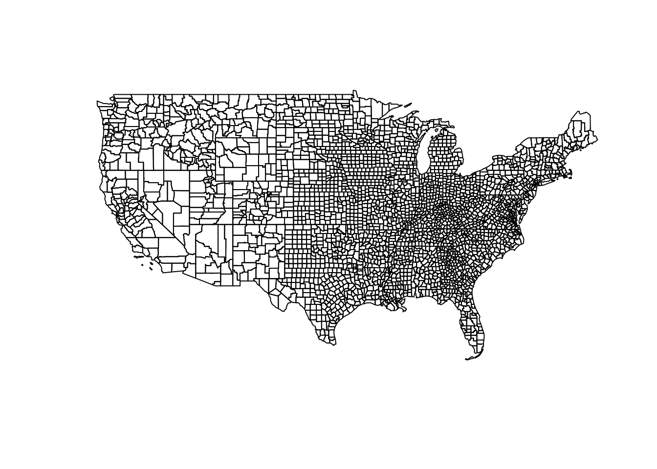
Active USGS gages
sites   = readRDS("shiny/usgs_sites.rds")
glimpse(sites)
#> Rows: 5,290
#> Columns: 4
#> $ name <chr> "Middlesex, MA", "Hampden, MA", "Hampshire, MA", …
#> $ siteID <chr> "01098530", "01176000", "01173500", "01127500", "…
#> $ geoid <chr> "25017", "25013", "25015", "09011", "09005", "330…
#> $ geometry <POINT [°]> POINT (-71.39745 42.32533), POINT (-72.2634…Core Leaflet functions
Auto generate basemap
basemap = function(){
  leaflet() %>%
    addProviderTiles('CartoDB.Positron') %>%
    setView(lat = 39, lng = -95, zoom = 3)
}
Example
basemap()Zoom to a county, given a GEOID
zoom_to_county = function(map, counties, FIP){

  shp    = filter(counties, geoid == FIP)
  bounds = as.vector(st_bbox(shp))

  clearGroup(map, 'shp') %>%
    addPolygons(data = shp,
                color      = "#003660",
                fillColor  = "#FEBC11",
                fillOpacity = .2,
                group = "shp") %>%
    flyToBounds(bounds[1], bounds[2], bounds[3], bounds[4])
}
Example
zoom_to_county(basemap(), counties, 25017)USGS functions
Wrapper for finding streamflow given a siteID
get_streamflow = function(siteID){
  readNWISdv(siteNumbers = siteID,
             parameterCd = '00060',
             startDate   = Sys.Date() - 365) %>%
    renameNWISColumns()
}
Example
flow = get_streamflow('01098530')
glimpse(flow)
#> Rows: 365
#> Columns: 5
#> $ agency_cd <chr> "USGS", "USGS", "USGS", "USGS", "USGS", "USGS", …
#> $ site_no <chr> "01098530", "01098530", "01098530", "01098530", …
#> $ Date <date> 2020-03-17, 2020-03-18, 2020-03-19, 2020-03-20,…
#> $ Flow <dbl> 158, 141, 170, 202, 191, 173, 174, 444, 471, 417…
#> $ Flow_cd <chr> "A", "A", "A", "A", "A", "A", "A", "A", "A", "A"…Network Linked Data Index function given a lat/lon
find_nldi  = function(x, y){
  findNLDI(location = c(x,y), nav = c('UM'),
           find = c("basin", "flowlines"), distance = 1000)
}
Example
nldi_out = find_nldi(-104.780837, 38.786796)

basemap() %>%
  addPolygons(data = nldi_out$basin) %>%
  addPolygons(data = nldi_out$UM_flowlines) %>%
  zoom_to_county(counties, '08041')
Where are we going?
We will use flexdashboard to generate the app.
If you know Rmarkdown basics, this will be intuitive for you!
The key new piece is that:
- Each Level 1 Header (#) begins a new page in the dashboard.
- Each Level 2 Header (##) begins a new column/row.
- Each Level 3 Header (###) begins a new box.
The app material can be found here