Getting Catchments
We can connect to the Lynker AWS s3 holdings to extract the refactored and aggregated catchments upstream of USGS gage ID: 01022500.
cats <- sf::read_sf("/vsis3/formulations-dev/CAMELS20/camels_01022500_2677104/spatial/hydrofabric.gpkg", "catchments")
Getting Elevation
Using the VRT produced for hydrofabric work and hosted via Github Pages, we can extract the needed 30m DEM (3DEP 1 - 1 arcsecond).
elev <- rast("/vsicurl/https://mikejohnson51.github.io/opendap.catalog/ned_USGS_1.vrt")

dem <- crop(elev, project(vect(cats), crs(elev)))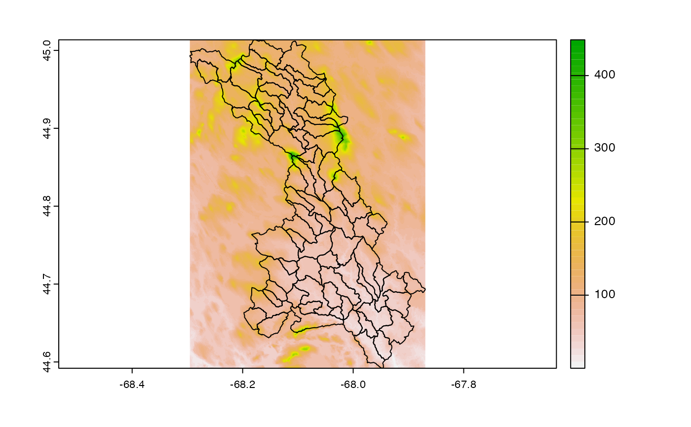
Compute TWI
Using the in-memory elevation data we can write a quick function to compute and save a TWI grid:
build_twi <- function(dem, outfile = NULL) {
  writeRaster(dem, "dem.tif", overwrite = TRUE)

  gdal_utils("warp",
    source = "dem.tif",
    destination = "dem_proj.tif",
    options = c(
      "-of", "GTiff",
      "-t_srs", "EPSG:5070",
      "-r", "bilinear"
    )
  )

  wbt_breach_depressions("dem_proj.tif", "dem_corr.tif")

  wbt_md_inf_flow_accumulation("dem_corr.tif", "sca.tif")
  wbt_slope("dem_proj.tif", "slope.tif")

  wbt_wetness_index(
    "sca.tif",
    "slope.tif",
    'fin.tif'
  )

  gdal_utils("translate",
         source = "fin.tif",
destination  = outfile,
options = c("-co", "TILED=YES",
"-co",  "COPY_SRC_OVERVIEWS=YES",
"-co",  "COMPRESS=DEFLATE"))


  unlink("dem.tif")
  unlink("dem_proj.tif")
  unlink("dem_corr.tif")
  unlink("sca.tif")
  unlink("slope.tif")
  unlink("fin.tif")


  return(outfile)
}

file <- build_twi(dem, outfile = "../private/twi.tif")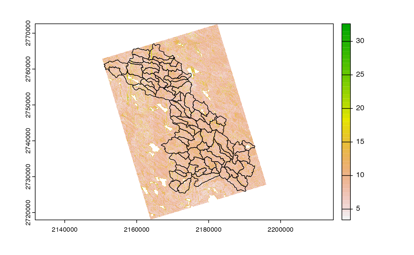
Summarize to catchment
We next compute a catchment level mean TWI using zonal.
o <- zonal::execute_zonal(file, cats, "ID", join = FALSE)
names(o)[2] <- "TWI"
head(o)
## ID TWI
## 1: cat-10 8.496850
## 2: cat-100 8.167785
## 3: cat-104 8.292524
## 4: cat-106 8.476784
## 5: cat-109 7.944167
## 6: cat-113 7.518617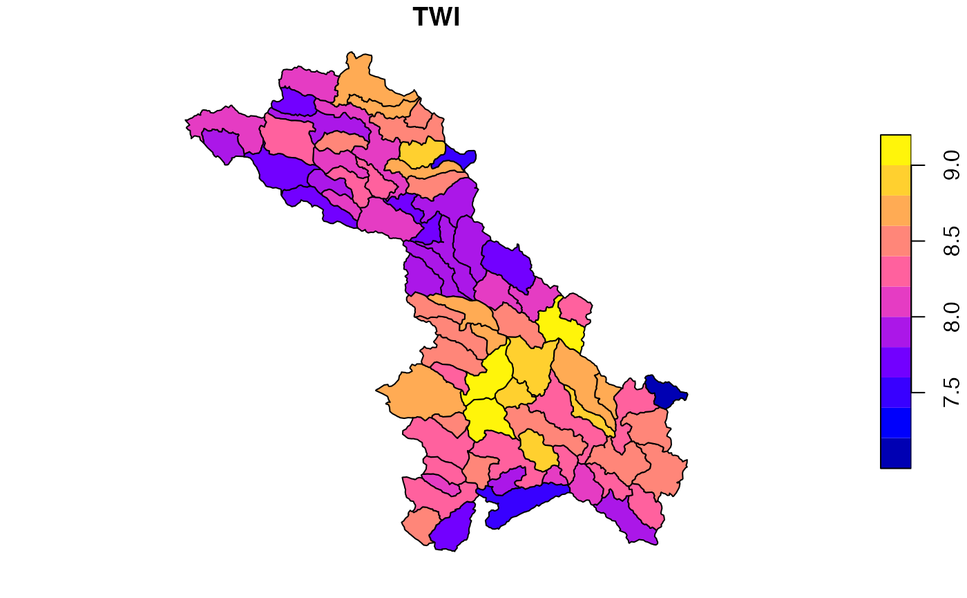
Map to NWM grid
The remaining workflow is representative of a process that might update frequently in a lumped formulation (e.g. soil moisture) creating the need to map values back to a common model grid. That is the reason a simple resample/regrid is not possible.
Materialize the grid:
nwm_1km <- materilize_grid(
  ext = ext(-2303999.62876143, 2304000.37123857, -1920000.70008381, 1919999.29991619),
  diminsion = c(3841, 4608),
  projection = 'PROJCS["Sphere_Lambert_Conformal_Conic",GEOGCS["GCS_Sphere",DATUM["D_Sphere",SPHEROID["Sphere",6370000.0,0.0]],PRIMEM["Greenwich",0.0],UNIT["Degree",0.0174532925199433]],PROJECTION["Lambert_Conformal_Conic"],PARAMETER["false_easting",0.0],PARAMETER["false_northing",0.0],PARAMETER["central_meridian",-97.0],PARAMETER["standard_parallel_1",30.0],PARAMETER["standard_parallel_2",60.0],PARAMETER["latitude_of_origin",40.000008],UNIT["Meter",1.0]];-35691800 -29075200 126180232.640845;-100000 10000;-100000 10000;0.001;0.001;0.001;IsHighPrecision'
)
Define Weight Map
(w <- weighting_grid(nwm_1km, cats, "ID"))## ID cell coverage_fraction
## 1: cat-3 4716637 0.07492989
## 2: cat-3 4716638 0.57502741
## 3: cat-3 4716639 0.04904574
## 4: cat-3 4720478 0.11056144
## 5: cat-3 4720479 0.98024553
## ---
## 1316: cat-222 4651331 0.79211766
## 1317: cat-222 4651332 0.55743623
## 1318: cat-222 4655171 0.07673281
## 1319: cat-222 4655172 0.06575897
## 1320: cat-222 4655173 0.16672505Define how to summarize
For this example we are computing a grouped mean. This is done by multiplying a value by its weight/covergage fraction and dividning bt the sum of the coverage_fraction.
Inject catchment values into cells…
dt <- merge(w, o, by = "ID")

# Apply areal.mean function over "TWI" grouped by cell
exe <- dt[, lapply(.SD, FUN = areal.mean, w = coverage_fraction),
          by = "cell",
          .SDcols = "TWI"
]

# Inject TWI data with into grid
nwm_1km[exe$cell] <- exe$TWI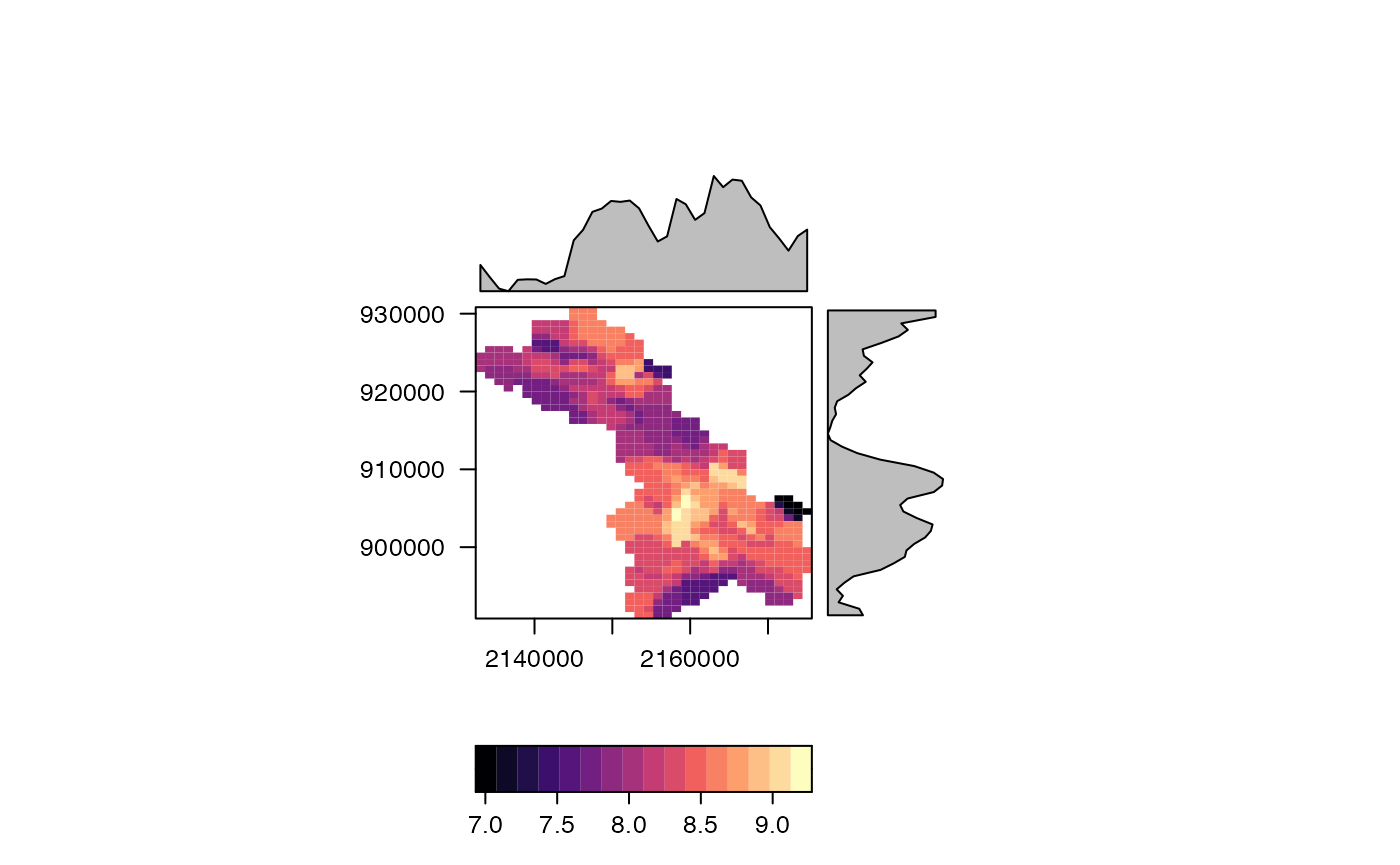
Distribute cell values into catchments
Say a new value was computed at the grid level and needs to be mapped back to the catchments. The “psuedo” value is:
-
TWI + a random number selected between 1 and 100.
Using the weight grid, this is a straight forward - table based process!
# Imagine this is a model time step updating the grid values...
nwm_1km[] = values(nwm_1km) + sample(1:100, ncell(nwm_1km), replace = T)

system.time({
  # Extract needed cell from layer (1) using the weight grid
  w$updated_value = nwm_1km[w$cell][,1]

  # Apply areal.mean function over "updated_value" grouping by ID
  exe <- w[, lapply(.SD, FUN = areal.mean, w = coverage_fraction),
    by = "ID",
    .SDcols = "updated_value"
  ]
})
## user system elapsed
## 0.002 0.001 0.003
head(exe)## ID updated_value
## 1: cat-3 61.27171
## 2: cat-8 61.28775
## 3: cat-10 75.12232
## 4: cat-15 59.54757
## 5: cat-16 57.18305
## 6: cat-18 58.01534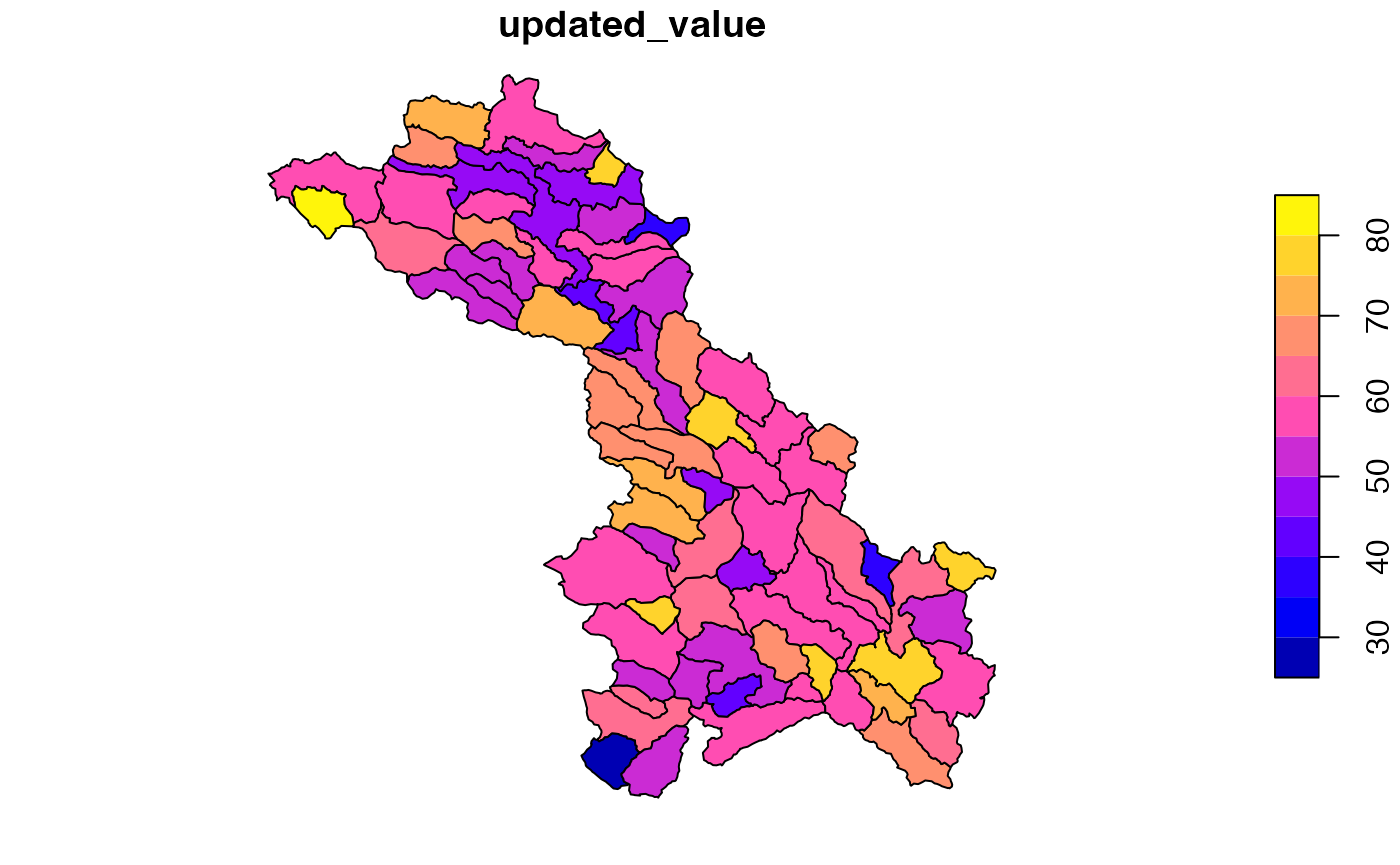
Does this scale?
So the question remains can this scale? I hope to show this with a quick naive, but more realisitic example of how the hydrofabric framework being build can support model engine goals:
Point to cloud environment
# AWS bucket location
  bucket = 'formulations-dev'
  subdir = 'hydrofabric/CONUS-hydrofabric/ngen-release/01a/2021-11-01/spatial'
local_pr = '/Users/mjohnson/github/zonal/to_build/pr_2020.nc'Build weight grid
Since this is “new” we will build the weight grid and upload it to s3. This only needs to be done once for each grid/hydrofabric pair.
write_parquet(weighting_grid(local_pr, cats, "ID"),
              "../private/gridmet_weights.parquet")

put_object(
    file      = "../private/gridmet_weights.parquet",
    object    = file.path(subdir, 'gridmet_weights.parquet'),
    bucket    = bucket,
    multipart = TRUE
  )

unlink("../private/gridmet_weights.parquet")
The produced weights parquet file is 814 KB… that’s it!
Grid –> catchments
Say we want aggregated catchment averages of the 4th day of GridMet rainfall. - Remote read the weights file - Partial read the forcing file - Apply areal.mean grouped by ID
system.time({
  w = read_parquet(file.path('s3:/',bucket, subdir, 'gridmet_weights.parquet'))

  w$rain = rast(local_pr)[[4]][w$cell]

  catchment_rainfall <- w[, lapply(.SD, FUN = areal.mean, w = coverage_fraction),
      by = "ID",
      .SDcols = "rain"
    ]
})
## user system elapsed
## 0.198 0.033 1.385
head(catchment_rainfall)## ID rain
## 1: cat-13581 1.659140
## 2: cat-711 0.000000
## 3: cat-13569 1.455351
## 4: cat-3 0.000000
## 5: cat-4 0.000000
## 6: cat-7 0.000000Naive hydrology
This is two generally show how hydrofabric attributes can be used in computation. We make a naive assumption that run off equals rainfall * %sand.
- Remote and partial read the
basin_attributesfile to get sand% - Compute catchment level “runoff”
system.time({
  sand = read_parquet(file.path('s3:/',bucket, subdir, ... = 'basin_attributes.parquet'),
                          col_select = c("ID", "sand-1m-percent"))

  model = merge(catchment_rainfall, sand, by = "ID")
  model$runoff = model$rain * model$`sand-1m-percent`
})
## user system elapsed
## 0.072 0.013 1.298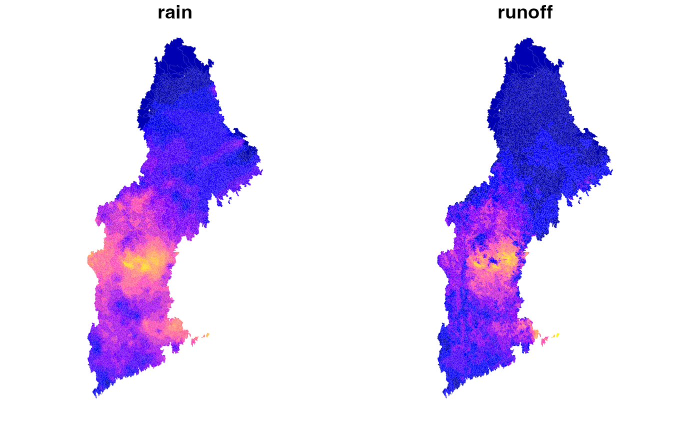
Catchment –> grid
If (for some reason) you want to take the catchment level “runoff” values, and map them back to the grid, you can do so…
system.time({
  dt <- merge(w, model, by = "ID")

  # Apply areal.mean function over "TWI" grouped by cell
  grid_runoff <- dt[, lapply(.SD, FUN = areal.mean, w = coverage_fraction),
            by = "cell",
            .SDcols = "runoff"
  ]
})
## user system elapsed
## 0.039 0.001 0.040
tmp = materilize_grid(local_pr, fillValue = 0)
tmp[grid_runoff$cell] <- grid_runoff$runoff
plot(tmp)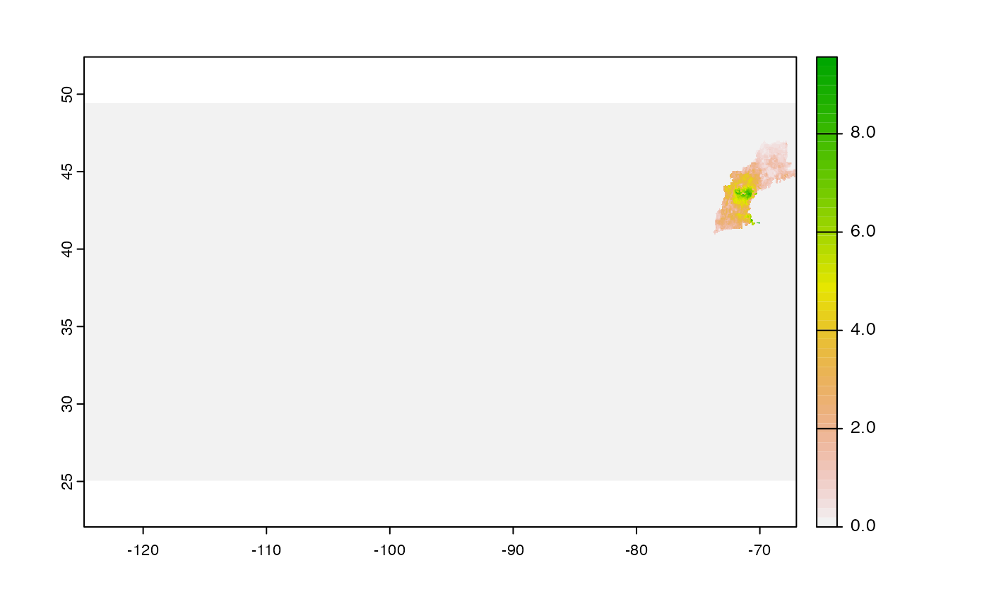
#plot(crop(tmp, project(vect(cats), crs(tmp))))