Historic Records

mikecp11@gmail.com

As part of a collaborative research effort, the multi-decadal historic simulation products from the NOAA National Water Model (versions 1.2, 2.0, and 2.1) have been reformatted and exposed through CUAHSI at the RENCI computing facility. This document outlines how to interact with this interface.

knitr::kable(get_nwm_meta(c(1.2, 2.0, 2.1)))

version	type	minDate	maxDate	ncml	varname
1.2	hydroshare	1993-01-01 00:00:00	2017-12-31 23:00:00	nwm_retro_full.ncml	feature_ids_v12
2.0	hydroshare	1993-01-01 00:00:00	2018-12-31 00:00:00	nwm_v2_retro_full.ncml	feature_ids_v20
2.1	USGS	1979-02-02 18:00:00	2020-12-31 00:00:00	nwm_v21_retro_full.ncml	feature_ids_v21

Data Extraction by …

Reanalysis data can be found with the readNWMdata function. The API requires users to specify NHD Common Identifier(s) (COMID), or NWIS site ID(s) for time series extraction.

NHD Catchment Identifier (COMID)

NWM reanalysis data can be extracted by NHD Catchment Identifier(s). The following code pulls the complete reanalysis data archive for COMID 17595383, a NHD reach near Goleta, California.

library(nwmTools)

system.time({
  flows = readNWMdata(comid = 17595383)
})
#>    user  system elapsed 
#>   0.133   0.063   1.108

head(flows)
#>      comid            dateTime flow_cms_v2.1
#> 1 17595383 1979-02-02 18:00:00          0.26
#> 2 17595383 1979-02-02 19:00:00          0.27
#> 3 17595383 1979-02-02 20:00:00          0.29
#> 4 17595383 1979-02-02 21:00:00          0.30
#> 5 17595383 1979-02-02 22:00:00          0.31
#> 6 17595383 1979-02-02 23:00:00          0.31
dim(flows)
#> [1] 367375      3

USGS NWIS Site Number

Alternatively, data can be extracted using USGS NWIS site ID(s).

system.time({
  flows = readNWMdata(siteID  = 11120000)
})
#>    user  system elapsed 
#>   2.846   0.194   4.028

head(flows)
#>      comid            dateTime   siteID flow_cms_v2.1
#> 1 17595429 1979-02-02 18:00:00 11120000          0.52
#> 2 17595429 1979-02-02 19:00:00 11120000          0.52
#> 3 17595429 1979-02-02 20:00:00 11120000          0.53
#> 4 17595429 1979-02-02 21:00:00 11120000          0.55
#> 5 17595429 1979-02-02 22:00:00 11120000          0.55
#> 6 17595429 1979-02-02 23:00:00 11120000          0.55
dim(flows)
#> [1] 367375      4

Query modification by …

The default behavior is to extract the complete, hourly time series in UTC, for the most current model version. Parameters allow data to be modified by data range, timezone and model version as follows:

date range

By default, the API extracts the complete flow record for each ID. This range can constrained by providing a startDate and/or endDate in the form of (“YYYY-MM-DD”).

system.time({
  utc <- readNWMdata(comid = 101, 
                     startDate = "2010-01-01", 
                     endDate   = "2010-01-31")
})
#>    user  system elapsed 
#>   0.090   0.047   0.459

# Check time dimensions
dim(utc)
#> [1] 744   3
range(utc$dateTime)
#> [1] "2010-01-01 00:00:00 UTC" "2010-01-31 23:00:00 UTC"
head(utc)
#>   comid            dateTime flow_cms_v2.1
#> 1   101 2010-01-01 00:00:00      9.650000
#> 2   101 2010-01-01 01:00:00      9.620000
#> 3   101 2010-01-01 02:00:00      9.599999
#> 4   101 2010-01-01 03:00:00      9.599999
#> 5   101 2010-01-01 04:00:00      9.610000
#> 6   101 2010-01-01 05:00:00      9.599999

time-zone

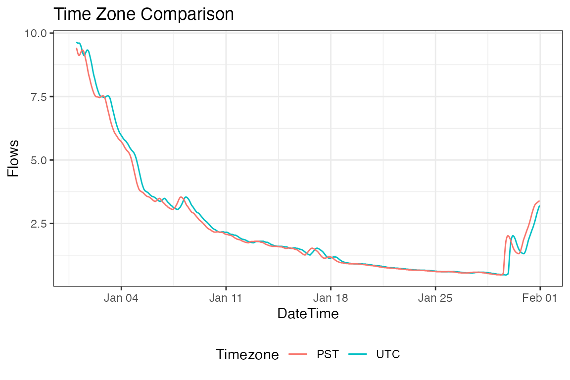
NWM output is recorded in UTC. Instead, users can specify a timezone. For our COMID in Goleta, California we can request data in US/Pacific time. Valid times zone can be found with OlsonNames().

pst = readNWMdata(comid = 101, 
                  startDate = "2010-01-01", 
                  endDate = "2010-01-31", 
                  tz = "US/Pacific")

# Check time dimensions
dim(pst)
#> [1] 744   3
range(pst$dateTime)
#> [1] "2010-01-01 00:00:00 PST" "2010-01-31 23:00:00 PST"
head(pst)
#>   comid            dateTime flow_cms_v2.1
#> 1   101 2010-01-01 00:00:00          9.42
#> 2   101 2010-01-01 01:00:00          9.32
#> 3   101 2010-01-01 02:00:00          9.22
#> 4   101 2010-01-01 03:00:00          9.15
#> 5   101 2010-01-01 04:00:00          9.12
#> 6   101 2010-01-01 05:00:00          9.13

Finally, we can plot the UTC return against the PST return:

Model versioning

The reanalysis product for versions 1.2, 2.0, and 2.1 of the NWM are available. By default the API extracts data from version 2.1, but all versions can be requested.

pst_vs = readNWMdata(comid = 101, 
                     startDate = "2010-01-01", 
                     endDate   = "2010-01-31",
                     tz        = "US/Pacific",
                     version =  c(1.2, 2.0, 2.1))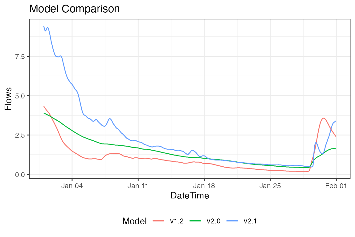

model version vs obs

In addition to extracting records from mulitple model runs, data can be appended from observation in the case a USGS gage ID is supplied:

system.time({
 data = readNWMdata(siteID = '01017000', 
            startDate = "2015-01-01",
            endDate = "2016-01-01",
            version = c(1.2, 2.0, 2.1),
            addObs = TRUE)
})
#>    user  system elapsed 
#>   6.775   0.416  17.347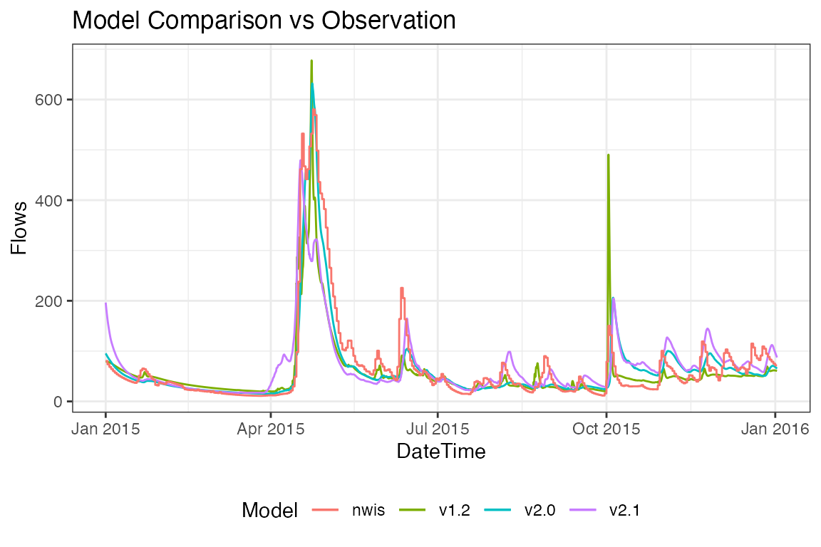

In section 2, we will look at how we can facilitate COMID and USGS NWIS discovery. In section 3 we will look at some techniques to handle operational data, and in section 4, we will look at time aggregations and splitting.