Time Aggregation{s}

Raw historic data comes in hourly time intervals. For many analyses, different time aggregates are needed (e.g. by year, by-month …). To ease repetative tasks, the nwmTools provides a split_time function and a family of aggregate_* functions.

Split-time

split_time in breaks the hourly dateTime into base temporal units. In addition to the basic year, month, day, and hour, the season, water year, and Day-of-Water Year (DOWY) are added:

# Get 5-years of data and split the time attribute
st = readNWMdata(comid = 101, 
                 startDate = "2005-01-01", 
                 endDate = "2009-12-31") |> 
  split_time("dateTime")

glimpse(st)
#> Rows: 43,824
#> Columns: 11
#> $ comid         <dbl> 101, 101, 101, 101, 101, 101, 101, 101, 101, 101, 101, 1…
#> $ dateTime      <dttm> 2005-01-01 00:00:00, 2005-01-01 01:00:00, 2005-01-01 02…
#> $ flow_cms_v2.1 <dbl> 2.23, 2.23, 2.22, 2.21, 2.19, 2.18, 2.18, 2.18, 2.17, 2.…
#> $ year          <dbl> 2005, 2005, 2005, 2005, 2005, 2005, 2005, 2005, 2005, 20…
#> $ month         <dbl> 1, 1, 1, 1, 1, 1, 1, 1, 1, 1, 1, 1, 1, 1, 1, 1, 1, 1, 1,…
#> $ day           <int> 1, 1, 1, 1, 1, 1, 1, 1, 1, 1, 1, 1, 1, 1, 1, 1, 1, 1, 1,…
#> $ hour          <int> 0, 1, 2, 3, 4, 5, 6, 7, 8, 9, 10, 11, 12, 13, 14, 15, 16…
#> $ season        <chr> "Winter", "Winter", "Winter", "Winter", "Winter", "Winte…
#> $ wy            <dbl> 2005, 2005, 2005, 2005, 2005, 2005, 2005, 2005, 2005, 20…
#> $ julian        <dbl> 1, 1, 1, 1, 1, 1, 1, 1, 1, 1, 1, 1, 1, 1, 1, 1, 1, 1, 1,…
#> $ DOWY          <dbl> 93, 93, 93, 93, 93, 93, 93, 93, 93, 93, 93, 93, 93, 93, …

Using the split time attributes, we can plot the hourly flow records by julien day, grouped by water-year:

ggplot(data = st, aes(x = DOWY, y = flow_cms_v2.1, color = flow_cms_v2.1)) + 
  geom_line(size = 1) +
  facet_grid(wy~.) +
  labs(y= "Daily Flow (cms)", x= "Day of Water Year", 
       title="Daily Discharge for COMID 101") +
  scale_color_viridis_c() +
  theme_minimal()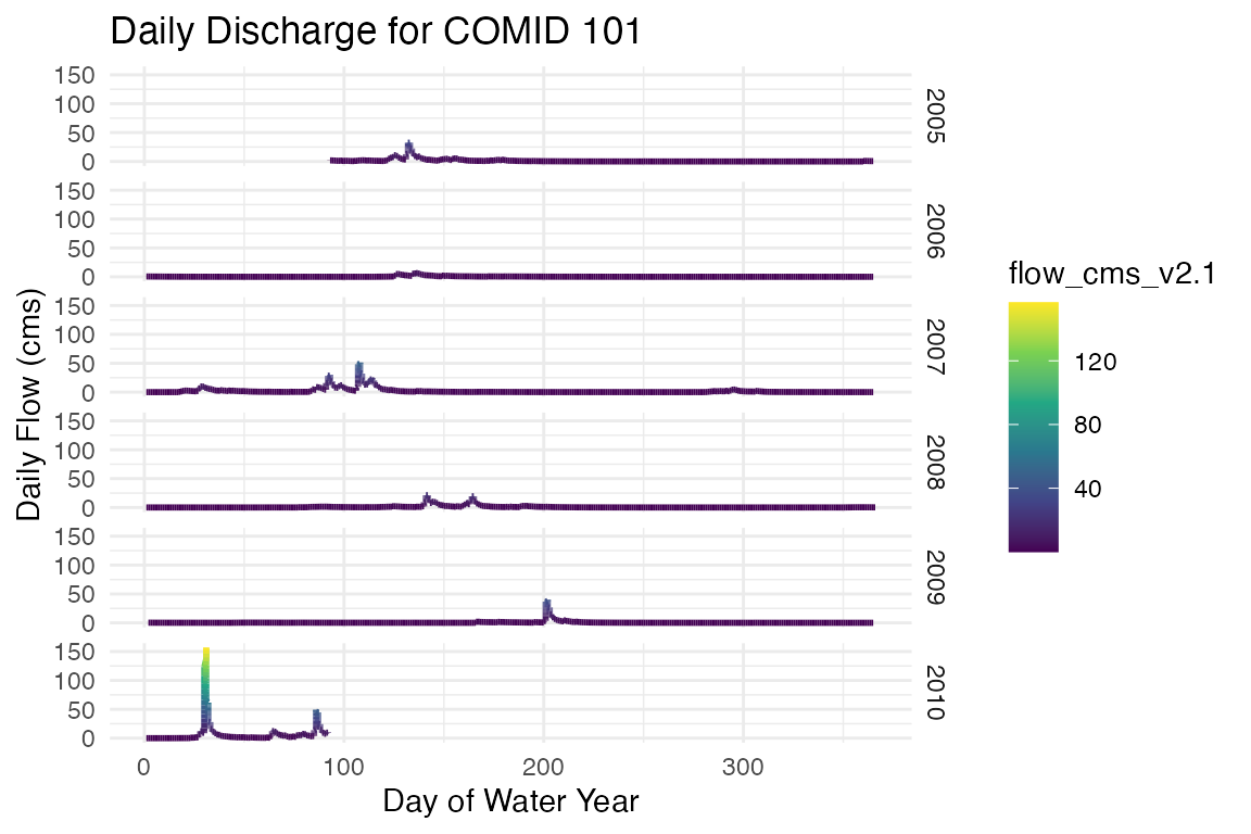

Aggregation

Often you might want to split and summarize your data, for example “average monthly flow” or “median annual flow”.

For these tasks, a family of aggregation methods allow users to define an temporal unit via the function name, and pass summarizing function(s) as parameters. Function names follow the pattern of aggregate_* where * represents the common date (and hydro-specific) symbols seen below.

Symbol	Aggregate
y	year
m	month
d	day of moth
doy	day of year
j	Julian day
s	season
wy	water year
dowy	day of water year

These symbols can be combined to provide useful, common aggregation patterns, 14 of these are included the package (some are shown below):

Aggregate Unit Symbol	Description
*_record	Entire Record
*_y	Year
*_m	Month
*_j	Julian Day
*_s	season
*_wy	Water Year
*_ym	Year and Month
*_yj	Year and Julian day
*_ymd	Day of the Year
*_ys	Year and Season
*_wym	Water Year and Month
*_wymd	Julian Day of the Water Year
*_wys	Water Year and Season
*_dowy	Day of Water Year

Examples

First lets grab some data for a COMID near Baton Rouge, LA along the Mississippi.

flows = readNWMdata(comid = 101)
glimpse(flows)
#> Rows: 367,375
#> Columns: 3
#> $ comid         <dbl> 101, 101, 101, 101, 101, 101, 101, 101, 101, 101, 101, 1…
#> $ dateTime      <dttm> 1979-02-02 18:00:00, 1979-02-02 19:00:00, 1979-02-02 20…
#> $ flow_cms_v2.1 <dbl> 3.02, 2.95, 2.89, 2.83, 2.79, 2.74, 2.70, 2.67, 2.63, 2.…

Single function

Using the flow data grabbed above, we might be interested in seeing the monthly mean flow rates. We can do this by passing the flow records to aggregate_m (m = month) and using mean as the function:

# Aggregate hourly flows to monthly averages by year
monthly = aggregate_m(flows, fun = mean)
glimpse(monthly)
#> Rows: 12
#> Columns: 4
#> $ comid         <dbl> 101, 101, 101, 101, 101, 101, 101, 101, 101, 101, 101, 1…
#> $ month         <dbl> 1, 2, 3, 4, 5, 6, 7, 8, 9, 10, 11, 12
#> $ flow_cms_v2.1 <dbl> 3.2080422, 3.0293795, 2.2485403, 1.3277797, 1.4821377, 1…
#> $ obs           <dbl> 30504, 28446, 31248, 30240, 31248, 30240, 31248, 31248, …

ggplot(data = monthly) + 
  geom_col(aes(x = factor(month), y = flow_cms_v2.1)) +
  labs(x = "Month", y = "Q (cms)", 
       title = 'Monthly Average') + 
  theme_bw()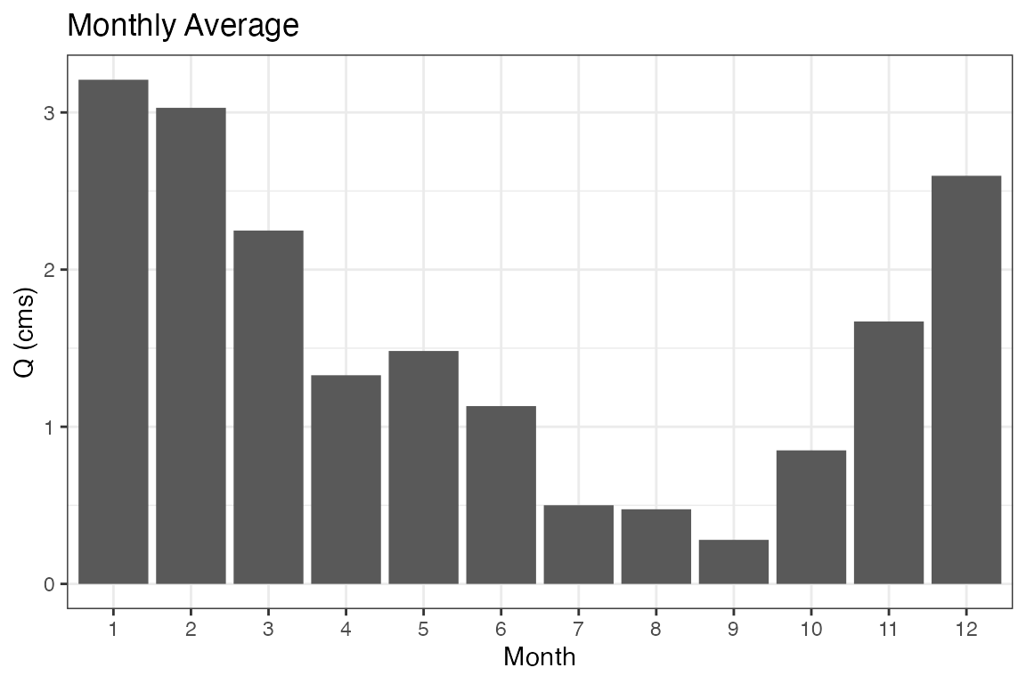

Alternatively we might be interested in the monthly variability in each year. We can do this by passing the flow records to aggregate_ym (ym = year,month) and using mean as the summarizing function:

# Aggregate hourly flows to monthly averages by year
ym = aggregate_ym(flows, fun = mean)
glimpse(ym)
#> Rows: 503
#> Columns: 6
#> $ comid         <dbl> 101, 101, 101, 101, 101, 101, 101, 101, 101, 101, 101, 1…
#> $ year          <dbl> 1979, 1979, 1979, 1979, 1979, 1979, 1979, 1979, 1979, 19…
#> $ month         <dbl> 2, 3, 4, 5, 6, 7, 8, 9, 10, 11, 12, 1, 2, 3, 4, 5, 6, 7,…
#> $ flow_cms_v2.1 <dbl> 5.27406337, 3.95766120, 3.80990269, 1.78446233, 3.922749…
#> $ obs           <dbl> 630, 744, 720, 744, 720, 744, 744, 720, 744, 720, 744, 7…
#> $ ym            <date> 1979-02-01, 1979-03-01, 1979-04-01, 1979-05-01, 1979-06…

ggplot(data = ym, aes(x = factor(month), y = flow_cms_v2.1)) + 
  geom_boxplot(alpha = .5, outlier.shape = NA) +
  labs(x = "Month", y = "Q (cms)", 
       title = 'By Month Variability') + 
  theme_bw()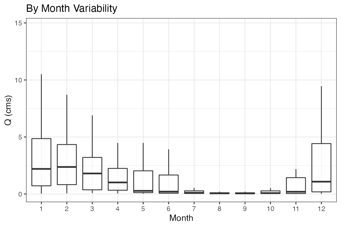

Multiple functions

So far we have only looked at passing mean to aggregate_* but multiple functions can also be passed as a vector. The following returns the seasonal (s) mean and standard deviation.

# Aggregate by season
seasons = aggregate_s(flows, fun = c('mean', 'sd'))
glimpse(seasons)
#> Rows: 4
#> Columns: 6
#> $ comid              <dbl> 101, 101, 101, 101
#> $ season             <chr> "Fall", "Spring", "Summer", "Winter"
#> $ flow_cms_v2.1_mean <dbl> 0.9324036, 1.6900479, 0.6976414, 2.9400717
#> $ obs_mean           <dbl> 91728, 92736, 92736, 90175
#> $ flow_cms_v2.1_sd   <dbl> 4.854523, 4.302834, 5.062546, 5.388558
#> $ obs_sd             <dbl> 0, 0, 0, 0

ggplot(data = seasons, aes(x = season, y = flow_cms_v2.1_mean)) +
  geom_errorbar(aes(ymin=flow_cms_v2.1_mean - flow_cms_v2.1_sd, ymax=flow_cms_v2.1_mean + flow_cms_v2.1_sd, width = .25)) +
  geom_point(color = "darkred", size = 2) +
  labs(x  = "Season", y = "Q(cms)", 
       title = "Seasonal mean +- sd")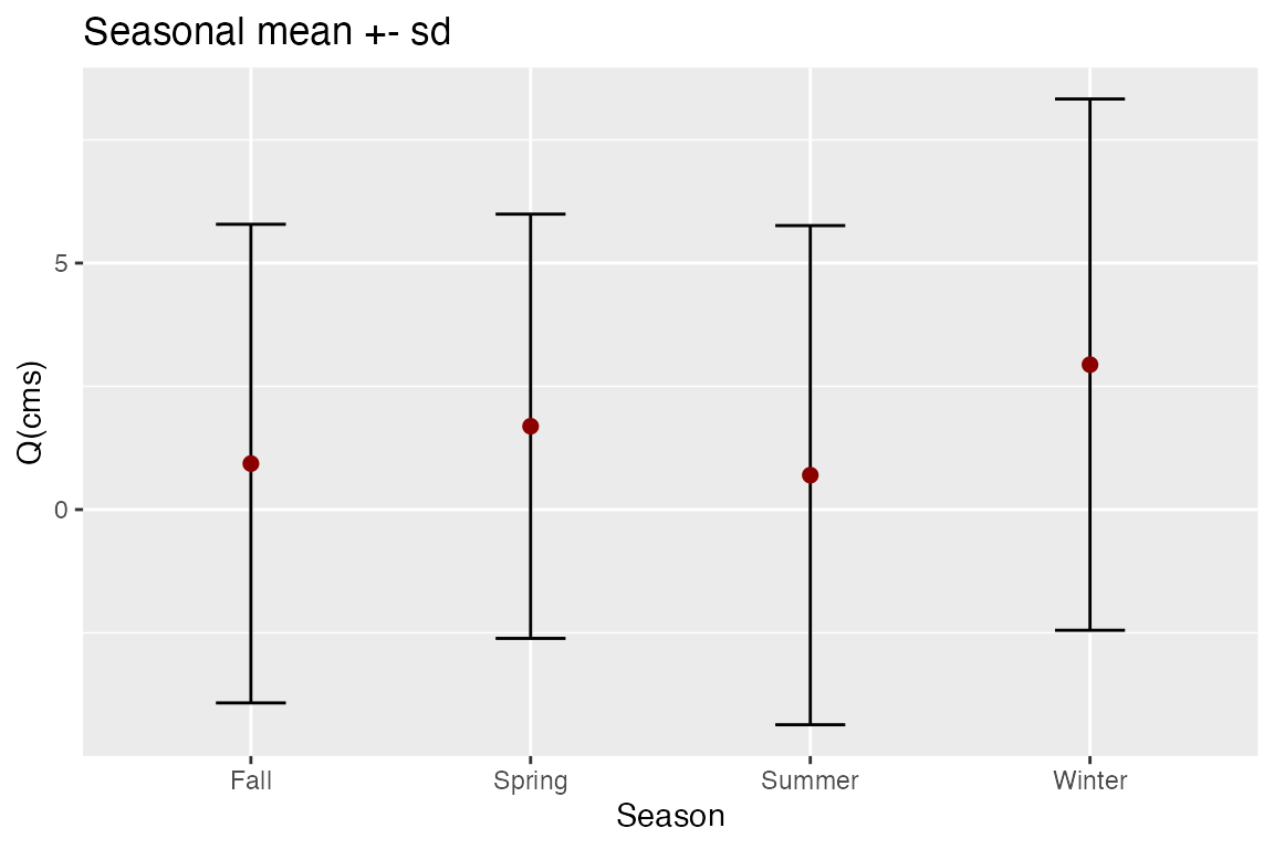

Custom Functions

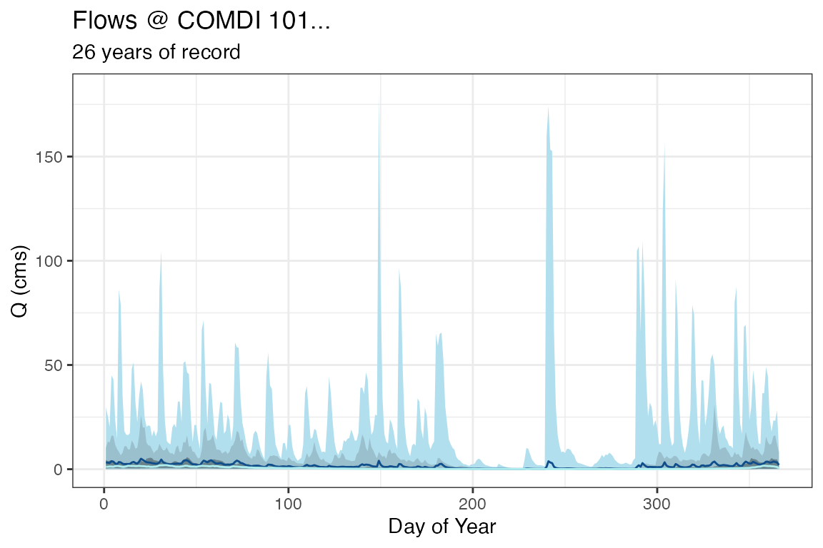
Equally important, you are not limited to base R functions. Instead you can pass any function to fun that works over a vector of streamflow elements. In the code below we ask for a number of percentiles along with some other summary statistics for every junlien day of the year: