library(zonal)
library(ggplot2)
library(dplyr)
library(sf)
library(tidyr)
library(terra)
library(paint)
In zonal categorical data is handled with
execute_zonal(..., FUN = 'freq') which computes the
relative proportion of a numeric class in each aggregation unit. In the
following we illustrate its use using a mosaiced 1km grid containing
MODIS 2019 land cover.
Grid
file = '2019-01-01.tif'
(r = rast(file))
## class : SpatRaster
## dimensions : 2896, 4616, 1 (nrow, ncol, nlyr)
## resolution : 1000, 1000 (x, y)
## extent : -2357000, 2259000, 277000, 3173000 (xmin, xmax, ymin, ymax)
## coord. ref. : +proj=aea +lat_0=23 +lon_0=-96 +lat_1=29.5 +lat_2=45.5 +x_0=0 +y_0=0 +datum=NAD27 +units=m +no_defs
## source : 2019-01-01.tif
## name : Land_Cover_Type_1
terra::plot(r)
Looking at the grid we can see in consists of 13367936 grid cells each with a 1000 meter by 1000 meter resolution. Additionally, there are 18 unique values in the grid (17 land cover and one nodata value).
Example 1: Basic Use
First, we want to identify the percent of each land cover within each
county in the USA Northeast. Doing this follows the same process as all
zonal workflows and requires (1) identifying the
aggregation units, (2) building a weight grid and (3) running the
intersection.
Define aggreation units
AOI  = AOI::aoi_get(state = "Northeast", county = "all")
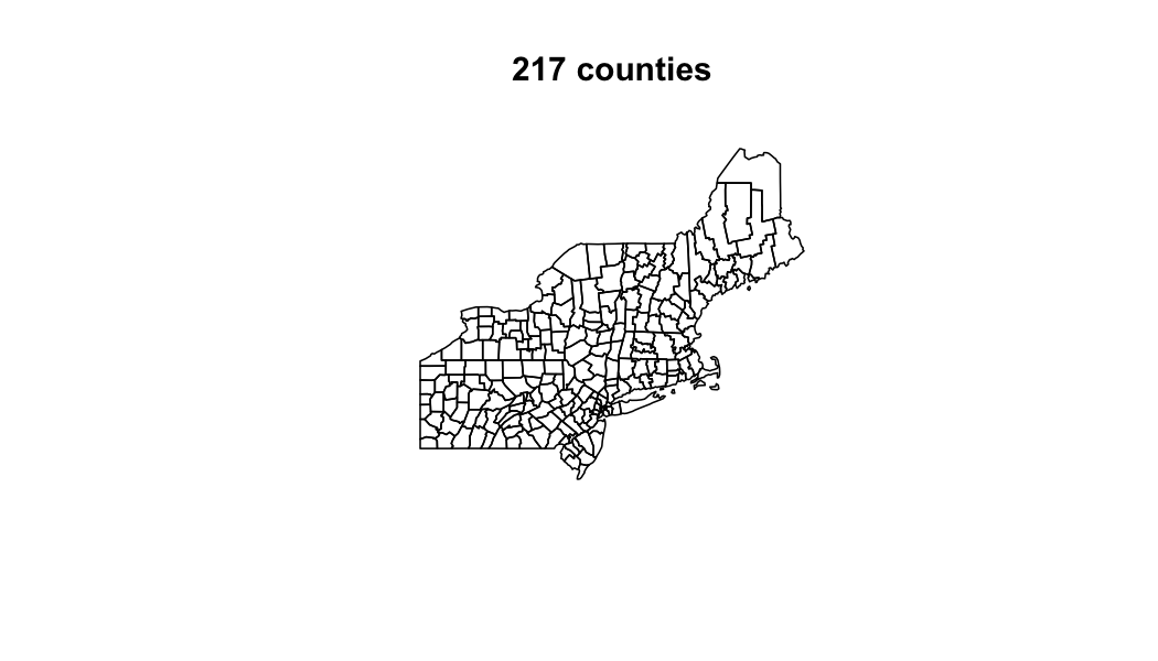
plot(AOI$geometry, main = paste(nrow(AOI), "counties"))
system.time({
  lc = execute_zonal(file, geom = AOI, ID = "geoid", FUN = "freq")
})
## user system elapsed
## 1.826 0.462 2.316
paint(lc)## sf [1997, 18]
## active geometry column: geometry (MULTIPOLYGON)
## crs: 4269 (NAD83)
## crs unit: degree
## geoid chr 09001 09001 09001 09001 09001 09001
## statefp chr 09 09 09 09 09 09
## countyfp chr 001 001 001 001 001 001
## countyns chr 00212794 00212794 00212794 00212794 0~
## affgeoid chr 0500000US09001 0500000US09001 0500000~
## name chr Fairfield Fairfield Fairfield Fairfie~
## namelsad chr Fairfield County Fairfield County Fai~
## stusps chr CT CT CT CT CT CT
## state_name chr Connecticut Connecticut Connecticut C~
## lsad chr 06 06 06 06 06 06
## aland dbl 1618664029 1618664029 1618664029 1618~
## awater dbl 549280913 549280913 549280913 5492809~
## state_name.1 chr Connecticut Connecticut Connecticut C~
## state_abbr chr CT CT CT CT CT CT
## jurisdiction_type chr state state state state state state
## value dbl 17 3 11 13 4 1
## percentage dbl 0.025932 0.002465 0.012004 0.257007 0~
## geometry sfc MPOLY 1,416B MPOLY 1,416B MPOLY 1,416~Example 2: Definining Classes
While the above works, calling on fields by their numeric ID is prone to error. Instead, this example shows how a reclassification table can be supplied to modify the column headings of the output table. A reclassification table tells us what each numeric value represents in a categorical raster. Below, we use a CSV file to define this mapping. The schema used is that one column must be named “from” - this is the existing data values, and one column must be named “to” - this is the desired column headings.
## data.frame [17, 2]
## from int 1 2 3 4 5 6
## to   chr evergreen_needle evergreen_broad deciduous_needle ~
Build a weight grid and execute intersection
system.time({
  lc = execute_zonal(file, geom = AOI, ID = "geoid", FUN = "freq", rcl = rcl)
})
## user system elapsed
## 1.808 0.454 2.285
paint(lc)## sf [1997, 18]
## active geometry column: geometry (MULTIPOLYGON)
## crs: 4269 (NAD83)
## crs unit: degree
## geoid chr 09001 09001 09001 09001 09001 09001
## statefp chr 09 09 09 09 09 09
## countyfp chr 001 001 001 001 001 001
## countyns chr 00212794 00212794 00212794 00212794 0~
## affgeoid chr 0500000US09001 0500000US09001 0500000~
## name chr Fairfield Fairfield Fairfield Fairfie~
## namelsad chr Fairfield County Fairfield County Fai~
## stusps chr CT CT CT CT CT CT
## state_name chr Connecticut Connecticut Connecticut C~
## lsad chr 06 06 06 06 06 06
## aland dbl 1618664029 1618664029 1618664029 1618~
## awater dbl 549280913 549280913 549280913 5492809~
## state_name.1 chr Connecticut Connecticut Connecticut C~
## state_abbr chr CT CT CT CT CT CT
## jurisdiction_type chr state state state state state state
## value chr water deciduous_needle wetlands urban~
## percentage dbl 0.025932 0.002465 0.012004 0.257007 0~
## geometry sfc MPOLY 1,416B MPOLY 1,416B MPOLY 1,416~Explore the data
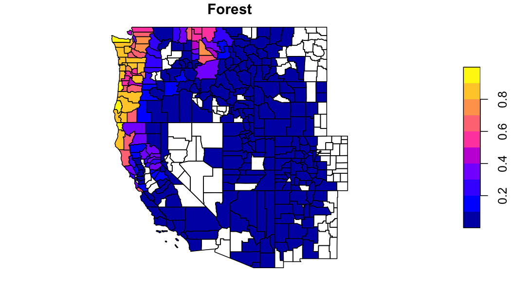
In the MODIS land cover scheme there are 5 classes loosly
representing forest. If wanted to aggregate these to a single forest
class, we can use the output zonal table.
forest = filter(lc, grepl('forest|broad|needle', value)) %>%
  group_by(geoid) %>%
  summarise(forest = sum(percentage)) %>%
  st_as_sf()

plot(forest['forest'], main = "Forest")
Compare with exactextractr
From the exactectractr vignettes there is an example to
compute class statistics using dplyr. Here we compare that
approach, to one supplemented with data.table, to
zonal with pre-computed weights, and to a single
zonal execution.
library(exactextractr)
library(data.table)

# exactextract with dplyr
exactextract_dplyr = function(file, AOI) {
  exact_extract(terra::rast(file), AOI, function(df) {
  df %>%
    mutate(frac_total = coverage_fraction / sum(coverage_fraction)) %>%
    group_by(geoid, value) %>%
    summarise(freq = sum(frac_total), .groups = "keep")
}, summarize_df = TRUE, include_cols = "geoid", progress = FALSE)
}

# exactextract with data.table
exactextract_dt = function(file, AOI){
  exact_extract(terra::rast(file), AOI, function(df) {
    dt = setDT(df)
    dt$frac_total = dt$coverage_fraction / sum(dt$coverage_fraction)
    dt[, .(freq = sum(frac_total, na.rm = TRUE)), by = .(value)]
  }, summarize_df = TRUE, include_cols = "geoid", progress = FALSE)
}

bnch <- bench::mark(
  iterations = 1, check = FALSE, time_unit = "s",
  exactextract_dplyr_out  = exactextract_dplyr(file, AOI),
  exactextract_dt_out     = exactextract_dt(file, AOI),
  zonal                   = execute_zonal(file, AOI, "geoid", FUN = "freq")
)

