zonal is an active package for intersecting vector aggregation units with large gridded data. While there are many libraries that seek to tackle this problem (see credits) we needed a library that could handle large gridded extents storing categorical and continuous data, with multiple time layers with both many small vector units and few large units.
The package offers 3 main options through a common syntax:
The ability to pregenerate weighting grids and applying those over large datasets distrbuted across files (e.g. 30 years of daily data stored in annula files). Rapid data summarization is supported by collapse and data.table.
Thin wrappers over pure exact_extract() when appropriate (e.g. calling a core
exactrextractrfunction)Flexible custom functions that are easily applied over multi layer files (e.g. geometric means and circular means)
Installation
You can install the development version of zonal with:
# install.packages("remotes")
remotes::install_github("mikejohnson51/zonal")
Example
This is a basic example that takes a NetCDF file containing a 4km grid for the continental USA and daily precipitation for the year 1979 (365 layers). Our goal is to subset this file to the southern USA, and compute daily county level averages. The result is a daily rainfall average for each county.
library(zonal)

AOI <- AOI::aoi_get(state = "south", county = "all")

d = rast("to_build/pr_2022.nc")

system.time({
  pr_zone <- execute_zonal(data = d,
                           geom = AOI,
                           ID = "fip_code",
                           join = TRUE)
})
#>    user  system elapsed
#>   5.150   0.766   5.963
Daily maximum mean rainfall in the South?
n = names(which.max(colSums(as.data.frame(pr_zone)[,grepl('precipitation', names(pr_zone))])))

ggplot(data = pr_zone) +
  geom_sf(aes(fill = get(n)), color = NA) +
  scale_fill_viridis_c() +
  theme_void() +
  labs(fill = "PR (mm)")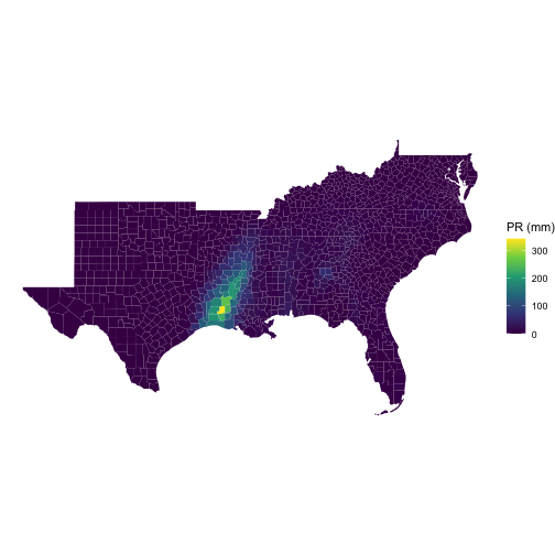
Timeseries of county with maximum annual rainfall
data <- pr_zone %>%
  as.data.frame() %>%
  slice_max(rowSums(select(., c(starts_with('mean'))))) %>%
  select(fip_code, starts_with('mean')) %>%
  pivot_longer(-fip_code, names_to = "day", values_to = "prcp") %>%
  mutate(day = as.numeric(gsub("mean.precipitation_amount_day.", "", day)))

head(data)
#> # A tibble: 6 × 3
#>   fip_code   day     prcp
#>   <chr>    <dbl>    <dbl>
#> 1 37175    44560 27.0
#> 2 37175    44561 17.2
#> 3 37175    44562  0.00712
#> 4 37175    44563  0
#> 5 37175    44564  0.0782
#> 6 37175    44565  3.15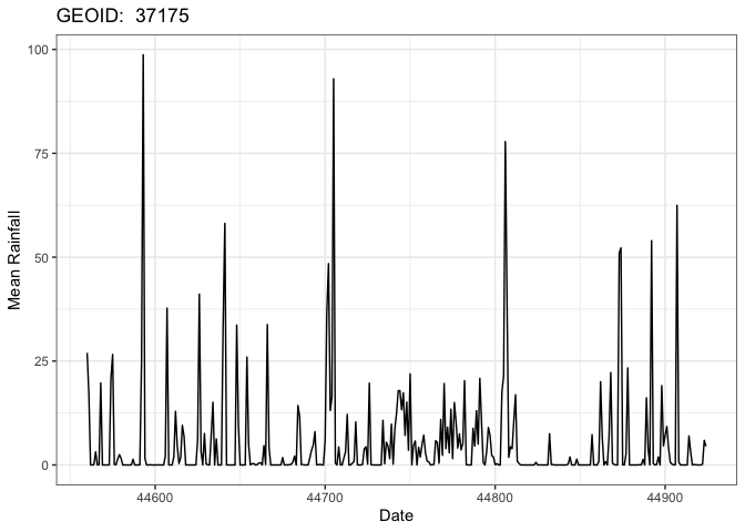
1km Landcover Grid (Categorical)
One of the largest limitations of existing utilities is the ability to handle categorical data. Here we show an example for a 1km grid storing land cover data from MODIS. This grid was creating by mosacing 19 MODIS tiles covering CONUS. The summary function for this categorical frequency is “freq”.
system.time({
  lc <- execute_zonal(data = rast("to_build/2019-01-01.tif"),
                      geom = AOI,
                      ID = "fip_code",
                      fun = "frac")
})
#>    user  system elapsed
#>   2.097   0.113   2.242
Zonal and opendap.catalog
Here lets look at a quick integration of the AOI/opendap.catalog/zonal family. The goal is to find monthly mean, normal (1981-2010), rainfall for all USA counties in the south.
library(climateR)

AOI <- AOI::aoi_get(state = "FL", county = "all")

system.time({
  data <- climateR::dap(
    URL = "https://cida.usgs.gov/thredds/dodsC/bcsd_obs",
    AOI = AOI,
    startDate = "1995-01-01",
    verbose = FALSE,
    varname  = "pr"
  ) |>
    execute_zonal(geom = AOI, ID = "fip_code", join = TRUE)
})
#>    user  system elapsed
#>   0.408   0.040   2.460

plot(data[grepl("mean", names(data))], border = NA)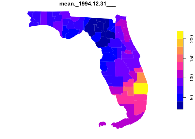
Getting involved
- Code style should attempt to follow the tidyverse style guide.
- Please avoid adding significant new dependencies without a documented reason why.
- Please attempt to describe what you want to do prior to contributing by submitting an issue.
- Please follow the typical github fork - pull-request workflow.
- Make sure you use roxygen and run Check before contributing.

