With a weight grid, zonal metrics can be computed. The four primary approaches use slightly different processes:
-
exactextractrleverages C libraries and an in memory raster and sf object. It works polygon-by-polygon to compute coverage’s and the weight table is computed within the function. -
intersectrutilizes NetCDF filepath and calculates all polygons timestep-by-timestep usingdata.table. A weight grid must be supplied. -
zonalworks from NetCDF or tif filepath and calculates all polygons and all time simultaneously usingdata.table. A weight grid must also be supplied.
The performance and comparison of these three approaches are shown below when the domain is large, and when (A) there a many thousands of polygons, and (B) when there a a few large polygon aggregation units.
Option 1: Intersectr:
The intersectr workflow for defining inputs for
execute_intersection are wrapping into a prep function
below:
intersectr_prep = function(file, geom, ID, variable){
  nc_coord_vars <- nc_coord_var(file)
  nc_coord_vars <- filter(nc_coord_vars, variable == !!variable)

  nc       <- open.nc(file)
  X_coords <- var.get.nc(nc, nc_coord_vars$X, unpack = TRUE)
  Y_coords <- var.get.nc(nc, nc_coord_vars$Y, unpack = TRUE)

  nc_prj <- nc_gm_to_prj(nc_grid_mapping_atts(file))

  cell_geometry = create_cell_geometry(X_coords = X_coords,
                         Y_coords = Y_coords,
                         prj = nc_prj,
                         geom = geom,
                         buffer_dist = 0.1, # Degrees
                         regularize = TRUE)

  data_source_cells <- st_sf(dplyr::select(cell_geometry, grid_ids))
  target_polygons   <- st_sf(dplyr::select(geom, !!ID))
  st_agr(data_source_cells) <- "constant"
  st_agr(target_polygons)   <- "constant"

  area_weights = calculate_area_intersection_weights(data_source_cells, target_polygons, allow_lonlat = TRUE)

  return(list(grid = cell_geometry, w = area_weights, x = nc_coord_vars$X, y = nc_coord_vars$Y, t = nc_coord_vars$T))
}
Option 2: exactextract:
The exacextract workflow for computing aggregate means
for a raster stack are wrapped below:
exactrextract_process = function(file, geom, ID){
  R.utils::withTimeout(
    exactextractr::exact_extract(raster::stack(file),
                                 geom,
                                 stack_apply = TRUE,
                                 fun = "mean",
                                 append_cols = ID,
                                 progress = FALSE),
  timeout = 180, onTimeout = "silent")
}
Spoiler Alert: This method can take an extremely long time when the polygon count is very high. As such, we are limiting the execution time to 180 seconds (three minutes). If a benchmark time indicates the process takes 180 seconds, it means the process was killed and not completed.
Option 3: zonal:
The zonal workflow for building a weight grid and
executing the areal averages can be executed with
execute_zonal.
library(zonal)Grid
The gridded data and aggregate units we are working with can be seen below:
file = 'pet_2020.nc'
(s = terra::rast(file))
## class : SpatRaster
## dimensions : 585, 1386, 366 (nrow, ncol, nlyr)
## resolution : 0.04167, 0.04167 (x, y)
## extent : -124.8, -67.04, 25.05, 49.42 (xmin, xmax, ymin, ymax)
## coord. ref. : lon/lat WGS 84 (EPSG:4326)
## source : pet_2020.nc
## varname : potential_evapotranspiration (pet)
## names : poten~43829, poten~43830, poten~43831, poten~43832, poten~43833, poten~43834, ...
## unit : mm, mm, mm, mm, mm, mm, ...Looking at the grid we can see in consists of 810810 grid cells each with a 0.0417 meter by 0.0417 meter resolution. Additionally, there are 366 unique time slices in the NetCDF file.
Example 1: HUC01
Our first example uses a hydrofabric developed for the Northeast USA.
geom <- read_sf('hydrofabric.gpkg', "catchments")
paint(geom)
## sf [18041, 4]
## active geometry column: geom (POLYGON)
## crs: 5070 (NAD83 / Conus Albers)
## crs unit: metre
## ID chr cat-1 cat-2 cat-4 cat-5 cat-6 cat-7
## area_sqkm dbl 12.457576 267.083595 8.319214 9.278138 60.577~
## toID chr nex-2 nex-3 nex-5 nex-6 nex-7 nex-8
## geom sfc POLY 2,024B POLY 9,064B POLY 1,656B POLY 1,81~In total we have 18,041 aggregation units to summarize over the 366 time steps. Both zonal and intersectr are designed to precompute a weight grid. Therefore we time how long it takes to do this using each method:
int_time_huc01 = system.time({
  intersectr_input = intersectr_prep(file,
                                     geom,
                                     ID = "ID",
                                     variable = 'potential_evapotranspiration')
})

zonal_time_huc01 = system.time({
  zonal_w = weighting_grid(file,
                           geom,
                           ID = "ID")
})
Next, we benchmark the time it takes to do the following: - run the
intersectr workflow with precomputed weights - run the
exactextractr workflow - run the zonal
workflow - run the zonal workflow with precomputed
weights
huc01_bnch <- bench::mark(
  iterations = 1, check = FALSE, time_unit = 's',
  intersectr_staged_weights = execute_intersection(nc_file = file,
                               variable_name = 'potential_evapotranspiration',
                               intersection_weights = intersectr_input$w,
                               cell_geometry = intersectr_input$grid,
                               x_var = intersectr_input$x,
                               y_var = intersectr_input$y,
                               t_var = intersectr_input$t,
                               start_datetime = NULL,
                               end_datetime = NULL),
  exactextractr            = exactrextract_process(file, geom, "ID"),
  zonal_full               = execute_zonal(file, geom, "ID"),
  zonal_staged_weights     = execute_zonal(file, w = zonal_w)
)
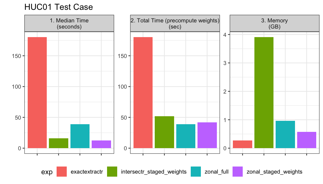
Overall when the polygon count is very high (~20,000), the zonal
aproach with precomputed weights and non precomputed weights performs
the best. Precomputing the weights save a significant amount of memory
in the process and ~4 seconds in total run time. These timings suggest
that 20 years of daily GridMet data could be computed for the ~20,000
catchments in about 11 minutes (~30 seconds * 20 year + ~15 seconds).
The intersectr approach requires way more memory despite
the precomputation of weights and takes about 3 times as long as zonal.
Lastly the exactextract methods timed out at the upper
limit of 180 seconds we prescribed.
Example 02: Florida Counties
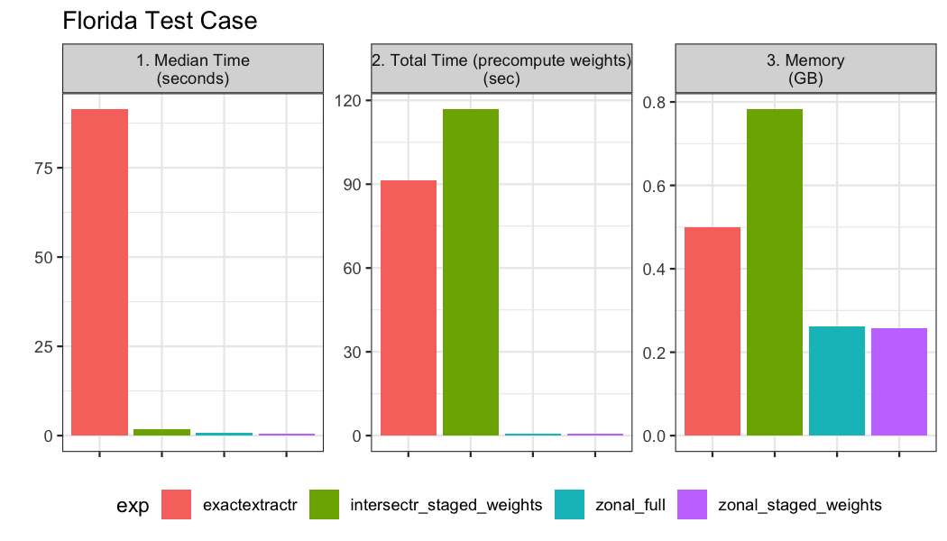
Our second example looks at the timings for an aggregation over a large area with a few aggregation units. The gridded data is the same as example 1, and the aggregate units can be seen below:
(florida <- AOI::aoi_get(state = "FL", county = "all"))## Simple feature collection with 67 features and 15 fields
## Geometry type: MULTIPOLYGON
## Dimension: XY
## Bounding box: xmin: -87.63 ymin: 24.5 xmax: -80.03 ymax: 31
## Geodetic CRS: NAD83
## First 10 features:
## statefp countyfp countyns affgeoid geoid name namelsad stusps
## 65 12 061 00307624 0500000US12061 12061 Indian River Indian River County FL
## 97 12 037 00306911 0500000US12037 12037 Franklin Franklin County FL
## 105 12 115 00295741 0500000US12115 12115 Sarasota Sarasota County FL
## 165 12 077 00308549 0500000US12077 12077 Liberty Liberty County FL
## 192 12 003 00306920 0500000US12003 12003 Baker Baker County FL
## 198 12 083 00306922 0500000US12083 12083 Marion Marion County FL
## state_name lsad aland awater state_name.1 state_abbr jurisdiction_type
## 65 Florida 06 1302272805 295509938 Florida FL state
## 97 Florida 06 1411498965 2270440522 Florida FL state
## 105 Florida 06 1440039085 1086628535 Florida FL state
## 165 Florida 06 2164099094 19582444 Florida FL state
## 192 Florida 06 1515738972 9686120 Florida FL state
## 198 Florida 06 4113993941 192281837 Florida FL state
## geometry
## 65 MULTIPOLYGON (((-80.88 27.8...
## 97 MULTIPOLYGON (((-85.21 29.7...
## 105 MULTIPOLYGON (((-82.65 27.3...
## 165 MULTIPOLYGON (((-85.12 30.2...
## 192 MULTIPOLYGON (((-82.46 30.5...
## 198 MULTIPOLYGON (((-82.53 29.2...
## [ reached 'max' / getOption("max.print") -- omitted 4 rows ]The same functions and timing from example 1 are computed:
int_time_fl = system.time({
  intersectr_input_florida = intersectr_prep(file, florida, ID = "geoid", variable = 'potential_evapotranspiration')
})

zonal_time_fl = system.time({
  zonal_w_florida = weighting_grid(file, florida, ID = "geoid")
})
fl_bnch <- bench::mark(
  iterations = 1, check = FALSE, time_unit = 's',
  intersectr_staged_weights = execute_intersection(nc_file = file,
                               variable_name = 'potential_evapotranspiration',
                               intersection_weights = intersectr_input_florida$w,
                               cell_geometry = intersectr_input_florida$grid,
                               x_var = intersectr_input_florida$x,
                               y_var = intersectr_input_florida$y,
                               t_var = intersectr_input_florida$t,
                               start_datetime = NULL,
                               end_datetime = NULL),
  exactextractr            = exactrextract_process(file, florida, "geoid"),
  zonal_full               = execute_zonal(file, florida, "geoid"),
  zonal_staged_weights     = execute_zonal(file, w = zonal_w_florida)
)