Methods
The first step in computing zonal statistics are the need to compute
a weight map that can be used to reallocate the gridded data with
respect to the percent overlapping each cell. There are two primary
packages that tackle this which include intersectr (which
uses areal as a back-end) and zonal which uses
exactextractr.
From the exactextractr documentation: “_Results from
exactextractr are more accurate than other methods because
raster pixels that are partially covered by polygons are considered. The
significance of partial coverage increases for polygons that are small
or irregularly shaped.”
The same premise applies to
intersectr/areal.
So, what is a weight grid?
A weight grid is unique to the aggregate units and grid its build
from. It contains columns documenting the X and Y indexes of each grid
cell along with the grid id. The X,Y are realtive to the entire grid,
while the grid ID is relative to subsetwithin the bounding domain of the
aggregations unit(s). Additionally the w stores the percent
overlap between the grid cell and the aggregation unit identified by the
ID column which is speified in the buildweighting_grid`
function. An example is shown below:
Option 1: Intersectr:
Setting up the data for a intersectr weights map
requires (1) computing a vector representation of the grid and (2)
intersecting this grid with the aggregation units to determine the
percent overlap or “coverage fraction”. Below the workflow from the
intersectr docs is wrapped in a function that requires a
NetCDF file path, a sf geometry set, an ID variable from
the geometries, and the variable to extract from the grid.
library(intersectr)
library(ncmeta)
library(RNetCDF)

intersectr_weights = function(file, geom, ID, var){
  nc_coord_vars <- nc_coord_var(file)
  variable_name <- var
  nc_coord_vars <- filter(nc_coord_vars, variable == variable_name)

  nc       <- open.nc(file)
  X_coords <- var.get.nc(nc, nc_coord_vars$X, unpack = TRUE)
  Y_coords <- var.get.nc(nc, nc_coord_vars$Y, unpack = TRUE)

  nc_prj <- nc_gm_to_prj(nc_grid_mapping_atts(file))

  cell_geometry = create_cell_geometry(X_coords = X_coords,
                         Y_coords = Y_coords,
                         prj = nc_prj,
                         geom = geom,
                         buffer_dist = 0.1, # Degrees
                         regularize = TRUE)

  data_source_cells <- st_sf(dplyr::select(cell_geometry, grid_ids))
  target_polygons   <- st_sf(dplyr::select(geom, !!ID))
  st_agr(data_source_cells) <- "constant"
  st_agr(target_polygons)   <- "constant"

  calculate_area_intersection_weights(
      data_source_cells,
      target_polygons, allow_lonlat = TRUE)
}
Option 2: Zonal
In zonal grid weights are calculated using
exactextractr as the back-end. The key function is
weighting_grid.
library(zonal)Use Cases
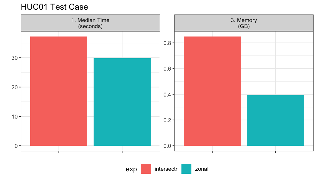
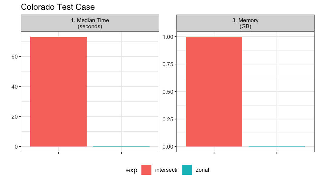
Here two motivating use cases are shown to compare the efficiency of these approaches. The first covers a large area but has many small aggregation units. The second covers a large area but has a few large polygon aggregation units. Each of these pose a unique set of demands with respect to how the calculation is performed.
Grid
The gridded data and aggregate units we are working with can be seen below and downloaded from here:
file = 'pet_2020.nc'
(s = terra::rast(file))
## class : SpatRaster
## dimensions : 585, 1386, 366 (nrow, ncol, nlyr)
## resolution : 0.04167, 0.04167 (x, y)
## extent : -124.8, -67.04, 25.05, 49.42 (xmin, xmax, ymin, ymax)
## coord. ref. : lon/lat WGS 84 (EPSG:4326)
## source : pet_2020.nc
## varname : potential_evapotranspiration (pet)
## names : poten~43829, poten~43830, poten~43831, poten~43832, poten~43833, poten~43834, ...
## unit : mm, mm, mm, mm, mm, mm, ...Looking at the grid we can see in consists of 810810 grid cells each with a 0.0417 meter by 0.0417 meter resolution. Additionally, there are 366 unique time slices in the NetCDF file.
Example 01: Many small aggregation units
Here, we look at an example with ~20,000 watersheds along the east coast.
geom <- st_make_valid(read_sf('hydrofabric.gpkg', "catchments"))

paint(geom)
## sf [18041, 4]
## active geometry column: geom (POLYGON)
## crs: 5070 (NAD83 / Conus Albers)
## crs unit: metre
## ID chr cat-1 cat-2 cat-4 cat-5 cat-6 cat-7
## area_sqkm dbl 12.457576 267.083595 8.319214 9.278138 60.577~
## toID chr nex-2 nex-3 nex-5 nex-6 nex-7 nex-8
## geom sfc POLY 2,024B POLY 9,064B POLY 1,656B POLY 1,81~In total we have 18,041 aggregation units to summarize over the 366 time steps.
bnch <- bench::mark(
  iterations = 1, check = FALSE, time_unit = "s",
  intersectr = intersectr_weights(file, geom, "ID", "potential_evapotranspiration"),
  zonal      = weighting_grid(s, geom, "ID")
)
Example 02: Few, large aggregation units
Here, we test aggregation the 4km gridded data to 64 counties in Colorado.
colorado  = AOI::aoi_get(state = "CO", county = "all")
paint(colorado)
## sf [64, 16]
## active geometry column: geometry (MULTIPOLYGON)
## crs: 4269 (NAD83)
## crs unit: degree
## statefp chr 08 08 08 08 08 08
## countyfp chr 125 111 009 099 027 043
## countyns chr 00198178 00198171 00198120 00198165 0~
## affgeoid chr 0500000US08125 0500000US08111 0500000~
## geoid chr 08125 08111 08009 08099 08027 08043
## name chr Yuma San Juan Baca Prowers Custer Fre~
## namelsad chr Yuma County San Juan County Baca Coun~
## stusps chr CO CO CO CO CO CO
## state_name chr Colorado Colorado Colorado Colorado C~
## lsad chr 06 06 06 06 06 06
## aland dbl 6123763559 1003660672 6617400567 4243~
## awater dbl 11134665 2035929 6142192 15317423 336~
## state_name.1 chr Colorado Colorado Colorado Colorado C~
## state_abbr chr CO CO CO CO CO CO
## jurisdiction_type chr state state state state state state
## geometry sfc MPOLY 888B MPOLY 904B MPOLY 920B MPOL~In total we have 64 aggregation units to summarize over the 366 time steps.
bnch2 <- bench::mark(
  iterations = 1, check = FALSE, time_unit = "s",
  intersectr = intersectr_weights(file, colorado, "name", "potential_evapotranspiration"),
  zonal      = weighting_grid(file, colorado, "name")
)